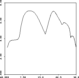
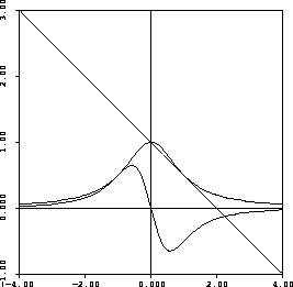
This is one where you have to sit down and do the graphing. As I said to several students in class, the important things to get are the points at which the slope is 0 (horizontal tangents), the points at which the slope is undefined, and the signs of the slopes between these points. Some relative magnitude of slopes would be nice, too, but that's in the bonus....
- find the domain.
- find the regions for which it is continuous, and differentiable.
- indicate what type of function it is.
- does it possess any symmetry?
-

-
domain:

- as a rational function, it is continuous and differentiable on its domain.
- rational function
- no symmetry (if it were symmetric it would need to have another removable discontinuity at -1).
-
domain:
-

-
domain:

- as a trigonometic function (cotangent), it is continuous and differentiable on its domain.
- trigonometic function
-
This is an odd function:

-
domain:
-

-
domain:
 , since

- This is a shifted absolute value function, which is continuous everywhere but not differentiable at 1 (the graph has a corner there).
- hifted absolute value function
- This function is neither odd nor even. It does possess symmetry about the line x=1.
-
domain:
![]()
Using the definition of the derivative, calculate its slope at x=1. Find the tangent line at that point, and draw it on your graph of f.
I could simply compute ![]() , but here's
, but here's ![]() :
:
![]()

![]()
Hence
![]()
The tangent line at ![]() is thus
is thus
![]()
![]()


-

We start by merely simplifying the expression of L:


Now the limit of the quotient is the quotient of the limits:

and the limit of the product is the product of the limits (while a limit of a composition of continuous function is continuous):


-

(Whoops! I left off a power of 2!) If the rational function has a positive limit, then the limit of the composition is the composition of the limits (this is the root law from section 2.3):

where we've used the fact that the limit of the quotient is the quotient of the limits. Now we can use the fact that the limit of a sum is the sum of the limits, and the limit of power functions, to write


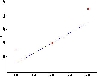
Graph the data, and estimate the rate of change in size at day 2 in two different ways:
- using the slope of a secant line, and
- fitting a function to the data, sketching the tangent line, and estimating the slope.
To begin with, we use the two points (1,3) and (3,9) to get a slope of the
secant line of ![]() for the point at x=2. We then draw
in the tangent line:
for the point at x=2. We then draw
in the tangent line:
I could draw a function which fits the data by hand also, and then estimate the slope using the standard ``rise over run'' formula.
As for estimating the slopes at the endpoints, we simply use the points themselves and their nearest neighbors: for example, at x=1, we'd estimate the slope using the two points (1,3) and (2,4), for a slope of 1.


