- Exercise #8, p. 227
- Interpolation (cont.)
- Mensa cereal quiz:
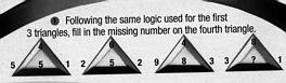
Modified Mensa cereal quiz: 4 6 4 8 5 2 9 3 1 2 3 1 1 1 1 ? Jen won the Mensa membership for following their linear reasoning to give the answer 6: the center point is half the sum of the corners. She probably would have had a harder time discovering the linear solution if there had been all 1's in the center: in that case, the coefficients are 0.1923, 0.0769, and -0.1538, so that
y = 0.1923*top + 0.0769*left - 0.1538*right
and the answer is 1.6154 (now I might give a mensa membership for that answer!). - Exercise #7, p. 226: How-to
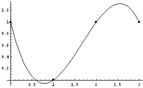
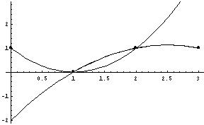
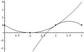
- Interpolating noisy data
- "[T]he human eye can be as good at curve fitting as any algorithm." p. 195.
- That said, here's the human eye algorithm:
- plot data carefully
- draw (by hand) the perceived trend
- pick reference points
- interpolate reference points
- Mensa cereal quiz:
- The statistics of simple regression
- Regression assumptions (p. 200):
- There is truly a (noisy) linear relationship between x and y.
- Residuals are independent
- Residuals are distributed as normal N(0, sigma)
- The F-Test
- Idea: compare power of model to explain variance to average. We'd like the mean sum of squares of the model to be much greater than that of the residuals, so we want F to be large (the model explains a lot).
- F=MSReg/MSRes
- Using the F table/ F distribution
- Simulation study results (p. 210-211)
- Standard errors and confidence intervals
- Parameter estimates are obtained; these estimates also have means and variances....
- Standard errors: standard deviation of the parameters, from a t-distribution (like a normal, only squatter)
- We get the same general information as the F-Test gives, except that we have a range of values we can use to represent the parameter, rather than a single number.
- Regression assumptions (p. 200):
- Example: Russ's Project (test evaluations) - simple linear regression
- Scatter plot and simple regression line (obvious linear
correlation!):
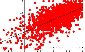
- Output:
Linear Regression:        Estimate        SE              Prob

Constant                 2.11374    (5.486696E-2)       0.00000
Variable 0               0.524759   (1.309028E-2)       0.00000

R Squared:               0.467971
Sigma hat:               0.297018
Number of cases:              1829
Degrees of freedom:           1827

  Source      df             SS              MS             F ratio

 Regression   1          141.77142       141.77142      1607.0250
 Residual     1827       161.17757       8.82197954E-2  Prob(f)=0.0000

 Lack of Fit  219        23.026099       .10514200      1.2237897
 Pure Error   1608       138.15147       8.59150918E-2  Prob(f)=0.2688
- Residuals: do they appear normal?
- Scatter plot and simple regression line (obvious linear
correlation!):
Note: