- Before we get started: I just have to share one story from my
Peace Corps days:

No student has ever worked harder than my brother-in-law Kpandja!
- We do have an exam Thursday through interpolation (it
will not go into differentiation, etc.). It will include
root-finding, as well. You should have a good handle on
chapters 3 and 5.
- You have an assignment due today. We'll go over any parts of it
you wish before we move forward.
- Do you all know Occam's
razor? A stronger form of it is one I prefer: "The simplest
consistent theory is the best." (and I apply it on #17,
p. 221).
- Any particular questions?
- Do you all know Occam's
razor? A stronger form of it is one I prefer: "The simplest
consistent theory is the best." (and I apply it on #17,
p. 221).
- Your projects are graded -- sorry about the delay. Some comments:
- Zach B.: Thank for citing your web references!
- Here's a "key".
- Newton's method
- You all seem pretty comfortable with this.
- Bisection
- What can we say about intervals containing more than two potential roots, leading to the choice of the root 0?
- What's a function of two variables doing in here?? One student said "I don't know how you would define and plot a function with two variables to give you an experimental answer."
- One student said "I'm not entirely sure what you mean about characterizing or symmetry." Let me explain.
- Fixed Point problem
- Is each method a valid fixed point scheme for this problem?
- What determines rates of convergence (and whether we can get convergence?
- Root finder comparison -- how to put the four schemes on a level playing field? Can we put them on a level playing field?
- Zach B.: Thank for citing your web references!
- Section 7.2: simple quadrature rules
We want to evaluate
You encountered the following rules back in calculus class, as you may recall:
- Trapezoidal
- Midpoint
- Simpson's Rule
We actually usually start with left- and right-rectangle rules, and then consider the trapezoidal rule as the average of these. Simpson's can be considered an average of the trapezoidal and the midpoint rules.
As the authors point out, the first two methods (trapezoidal and midpoint) can be considered integrals of linear functions.
The trapezoidal method is the integral of a linear interpolator of two endpoints, and midpoint is the integral of the constant function passing through -- well, the midpoint of the interval!
This illustrates one important different application of these two methods:
- trapezoidal requires the endpoints;
- midpoint doesn't require the endpoints.
These methods are both examples of what are called "Newton-Cotes methods" -- trapezoidal is a "closed" method, and midpoint is "open".
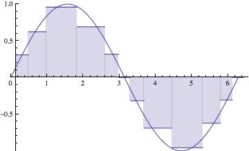
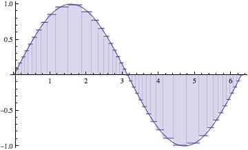
In the end we paste these methods together on a "partition" of the interval of integration -- that is, multiple sub-intervals, on each one of which we apply the simple rule. This pasted up version is called a "composite" rule.
We're going to start by assuming a partition of the intervalthat is equally spaced. But in the end, we should let the behavior of
help us to determine the the partition of the interval:


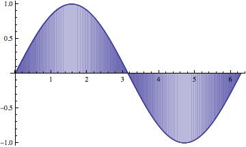
The maximum subinterval width ( ) goes to zero. The partition gets thinner and thinner, as the number of subintervals (n) goes to
.
The approximations get better and better, of course, as n) goes to.
Notice that the larger subintervals occur where the function isn't changing as rapidly.
This scheme would be called "adaptive", adapting itself to the function being integrated. That's what we're going to shoot for. - The derivation of the standard methods is carried out on pages
269-275, much as you might have seen before in calculus class.
Of particular interest in this section is the authors' very beautiful demonstration that Simpson's rule is the weighted average of the trapezoidal and midpoint methods.
In particular, that the midpoint method is twice as good as the trapezoidal method, and that the errors tend to be of opposite sign. This analysis is based off of an approximating parabola (see Figure 7.10, p. 271).
In that figure that bottom line is the tangent line at the midpoint (as suggested in paragraph above). The slope of that tangent line is actually equal to the slope of the secant line there, for a parabola. So the difference in those two slopes indicates the extent to which a parabolic model for
fails on that section.