Day 23 in Mat360

Today:

• Announcements:
  • Project 1 is graded (I'll email comments to each group). Every group received either a 7, a 7.5, or an 8 out of 8. However that was after a "curve" of .5 points. So no group was perfect -- how sad!:)
    • I'll be a little tougher in your next iteration, in the following ways:
      1. Your project should look like a group project -- not like it's stitched together by three or four different individuals.
      2. Make it look more professional.
         • Some of your notebooks didn't even have your names in them (or they were cleverly concealed).
         • Break things into clear sections. Clearly indicate results (summarize).

    • Some greatest hits:
      1. Zach, et al
      2. Zach, et al; Alyssa, et al
      3. Zach, et al and Alyssa, et al -- gold stars; Mangus, et al -- great graphic on g2 failure to converge
      4. Everyone fell down a little; the problem primarily was the use of a single starting point. You need to consider how they do on several different starting points. See my example code for one way to do that.

  • Homework is graded.
    • p. 190, #1, 2 ("Don't Simplify!"); #8 (Michael M.)
    • p. 206, #2 (Michael W.) and #4 (Lauren)
    • p. 221, #7, 10 (Joey -- conclusion)

  • You have a "knowledge demonstration opportunity" on Thursday. It will cover interpolation and root-finding techniques.
    • Look over your homeworks on roots and interpolation.
    • Look over the projects.
    • Look over class notes for featured ideas.
    • Read your book: all of Chapter 3, and Sections 5.0-5.6 in Chapter 5 (with minor omissions, such as Chebyshev nodes, and 5.5.2 Plotting)

    • Bring a calculator.

  • On Thursday, as you walk out of the exam, you'll receive your second project and group assignment (and three weeks to do it), and a homework assignment over differentiation.

• Today:
  • I'll start with questions on Root-Finding and Interpolation.

  • More Chapter 7 (numerical differentiation and integration).
    • Section 7.1: numerical differentiation
      • We begin with the one-sided forward-difference formula, which comes out of the most important definition in calculus (the limit definition of the derivative) by simply dropping the $h$:
        $f'(a)\approx\frac{f(a+h)-f(a)}{h}$

        The authors define the truncation error as the difference of the approximation and the true value:

        $\frac{f(a+h)-f(a)}{h}-f'(a)$

        and the power of $h$ on this error will be called the order of accuracy.

        The text illustrates this in Figure 7.1, p. 256, as the slope of a secant line approximation to the slope of the tangent line (the derivative at $x=a$).

        We explore the consequences using the Taylor series expansion:

        $f(a+h)=f(a)+hf'(a)+\frac{h^2}{2!}f''(a)+\frac{h^3}{3!}f'''({\xi}(h))$

        What is the order of accuracy of this method?

        We call this a forward definition, because we think of $h$ as a positive thing. It doesn't have to be however; but we define the backwards-difference formula (obviously closely related) as

        $f'(a)\approx\frac{f(a)-f(a-h)}{h}$

        which comes out of

        $f(a-h)=f(a)-hf'(a)+\frac{h^2}{2!}f''(a)-\frac{h^3}{3!}f'''({\xi}(h))$

      • Compare these "lop-sided" schemes with the centered-difference approximation:
        $f'(a)\approx\frac{f(a+h)-f(a-h)}{2h}$

        which we can again attack using Taylor series polynomials. What is the order of accuracy of this method?

        We can also derive it as an average of the two lop-sided schemes! We might then average their error terms to get an error term. However, what do you notice about that error term?

      • This is really a good time to make use of our tools from linear algebra, however. Let's take another crack at deriving these methods, but from the LA perspective, and see how matrices can make our problem so much easier, and allow us to generalize these simple ideas quite simply.

      • Now one thing you might think is that, by making $h$ smaller, you'll get better results. This is not necessarily so, and we should make clear that there are "competing interests" (or errors).

        Let's think about computing with error.

        It will turn out that the truncation error of a scheme like these will look like

        $E = \left| \frac{h}{2}f''(\xi) + \frac{e(x_0+h)-e(x_0)}{h} \right| \le \frac{M|h|}{2} + \frac{2 \epsilon}{h}$

        where $M>0$ is a bound on the derivative of interest on the interval of interest (second in this case), and $\epsilon>0$ is a bound on the size of a truncation or round-off error.

      • Richardson Extrapolation
        • For the forward difference
        • For the second derivative

    • Section 7.2: simple quadrature rules

      We want to evaluate

      $\int_a^bf(x)dx$

      You encountered the following rules back in calculus class, as you may recall:

      • Trapezoidal
      • Midpoint
      • Simpson's Rule

      We actually usually start with left- and right-rectangle rules, and then consider the trapezoidal rule as the average of these. Simpson's can be considered an average of the trapezoidal and the midpoint rules.

      As the authors point out, the first two methods (trapezoidal and midpoint) can be considered integrals of linear functions.

      The trapezoidal method is the integral of a linear interpolator of two endpoints, and midpoint is the integral of the constant function passing through -- well, the midpoint of the interval!

      This illustrates one important different application of these two methods:

      • trapezoidal requires the endpoints;
      • midpoint doesn't require the endpoints.
      Question: How might that be useful?

      These methods are both examples of what are called "Newton-Cotes methods" -- trapezoidal is a "closed" method, and midpoint is "open".

      In the end we paste these methods together on a "partition" of the interval of integration -- that is, multiple sub-intervals, on each one of which we apply the simple rule. This pasted up version is called a "composite" rule.

      We're going to start by assuming a partition of the interval $[a{,}b]$ that is equally spaced. But in the end, we should let the behavior of $f$ help us to determine the the partition of the interval: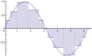

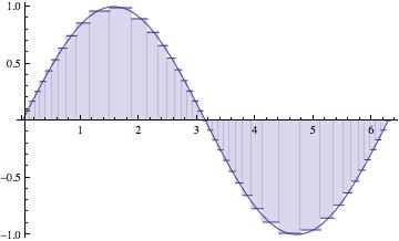
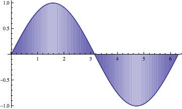
      The maximum subinterval width ($||{P}||$) goes to zero. The partition gets thinner and thinner, as the number of subintervals (n) goes to $\infty$. The approximations get better and better, of course, as $n \longrightarrow \infty$. Notice that the larger subintervals occur where the function isn't changing as rapidly. This scheme would be called "adaptive", adapting itself to the function being integrated. That's what we're going to shoot for.

    • The derivation of the standard methods is carried out on pages 269-275, much as you might have seen before in calculus class.

      Of particular interest in this section is the authors' very beautiful demonstration that Simpson's rule is the weighted average of the trapezoidal and midpoint methods.

      In particular, that the midpoint method is twice as good as the trapezoidal method, and that the errors tend to be of opposite sign. This analysis is based off of an approximating parabola (see Figure 7.10, p. 271).

      In that figure that bottom line is the tangent line at the midpoint (as suggested in paragraph above). The slope of that tangent line is actually equal to the slope of the secant line there, for a parabola. So the difference in those two slopes indicates the extent to which a parabolic model for $f$ fails on that section.

• Notes from Class:
  • Interpolation (showing Joey!) and differentiation