This makes sense, because when the hare become numerous, the lynx find life really good, and prosper. Then, when the lynx prosper too much, they prey on too many hare, and the hare population drops precipitously.
And so it goes....
Now let's get started....
- If you've not yet gotten your account set up with InsightMaker, do that first.
- Then visit Logistic-Growth,
which we cloned before. If you have already cloned it, you'll find it
from your home page under your models; otherwise, "Clone Insight" is in the top
right corner of your screen -- do so.
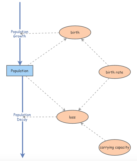
You should have something that looks like this:

When we talked about differential equations before spring break, we looked at the logistic differential equation, \[ \frac{dy}{dt}=b y\left(1-\frac{y}{K}\right) \] which we think of as the prey equation.
We started with the birth part of that, and talked about the general method of solving differential equations: stare at them until a solution comes to you! So the solution to this DE (differential equation), \[ \frac{dy}{dt}=b y \] is given by solving the problem "whose derivative function is simply a multiple of the function itself?" And the answer is an exponential function, \[ y(t)=Ce^{bt} \] Now things get a little more complicated when we throw in the death term. If we try the same trick, and solve it separately, well we can do that one by inspection, too: \[ \frac{dy}{dt}=\frac{-b y^2}{K} \] Whose derivative function is the proportional to the negative square of the function? That one is also not too hard: \[ y(t)=-\frac{K}{bt} \] But we can't just put these two functions together to get the solution to the logistic DE. In fact, the general solution of the logistic equation, in the case where $y_0 \ne 0$, is \[ y(t)=\frac{K}{1-e^{-(bt+Kc)}} \] with \[ y(0)=\frac{K}{1-e^{-Kc}}=y_0 \ \implies \ c = \frac{\ln\left(1-\frac{K}{y_0}\right)}{-K} \] So we can rewrite \[ y(t)=\frac{K}{1-e^{-bt}e^{-Kc}} =\frac{K}{1-\left(1-\frac{K}{y_0}\right)e^{-bt}} =\frac{y_0K}{y_0-(y_0-K)e^{-bt}} \]
In this lab, you will interact with your InsightMaker model. Start with the following parameters:
carrying capacity $K=90$ birth rate $b=.3$ initial population $y_0=10$ For "Settings", make sure that you're running in Years, 0 to 15, with RK4, and with Simulation Time Step of 0.1.
- Now to the stuff that you're going to report back to me:
- Create a Word file (or similar) for your results. Hit "Simulate",
and (find some way to) paste the graph into the Word file. (On my mac
I'm having trouble getting the image saved right, or viewed right, so
I'm reduced to taking a picture of it with screen capture.)
What's going on with the population over the 15 years? How is it changing?
- Now we want to investigate how the solution (the population over
time) changes as the initial population changes:
Describe how the behavior of the solution changes qualitatively as a function of time, as the initial value changes from 0 to $2K$ (twice the carrying capacity).
In particular, indicate the intervals where the solution is qualitatively similar (in particular, there is a special value of the initial population between 0 and $K$ that you will need to determine). Describe the behavior for that interval. Include any special cases (e.g. $y_0=K$, $y_0=0$).
Try at least $y_0=.1K$, $y_0=.8K$, $y_0=K$, $y_0=1.2K$, $y_0=2K$.
If you keep each of these simulation open, you can use the "Tools" menu to "Compare Results" -- show all the simulations in a single plot. That would be a good way to show me all of your results.
The teachable moment: Notice that we use $K$ as a sort of "standard unit" of population: \[ \frac{dy}{dt}=b y\left(1-\frac{y}{K}\right) \] If you multiply left and right by $\frac{1}{K}$, you get \[ \frac{d}{dt}\left(\frac{y}{K}\right)=b \frac{y}{K} \left(1-\frac{y}{K}\right) \] Then define a new dimensionless quantity, $w(t)=\frac{y}{K}$ (the population relative to its carrying capacity), and we get the simpler equation \[ \frac{dw}{dt}=b w (1 - w) \] which one can study instead. It contains all the dynamics of the original, with slightly less complexity. This is a standard trick in mathematics.
One further trick, and we've really simplified things: divide both sides by $b$: \[ \frac{dw}{d(bt)}= w (1 - w) \] and redefine the dimensionless time unit, to $\tau=bt$: \[ \frac{dw}{d\tau}= w (1 - w) \] $\tau=1$ when $t=\frac{1}{b}$: so if $b=.5/year$, then $\tau=1$ when $t=2$. So the larger $b$ (the greater the birthrate), the shorter time $t$ to give $\tau=1$.
This equation, as simple as possible, contains all the dynamics (all the ways the population can behave), while masking the "trivialities"; but it kind of hides the physical aspects of the problem. So it's easy to study, but harder to interpret: alas, you can't have it all!:)
I illustrate this simplest form in another InsightMaker model. If you check out that one, you'll see that there's really only one "important" parameter: the starting population, relative to the carrying capacity.
- Return the parameter values back to their original starting
values. For "Settings", increase the number of Years, from 0 to 30.
Change the "Population Decay" "Flow Rate" to
[loss]*(1+.3*sin(2*pi*(Years())))
and note how the solutions change.
(Why might a periodic death flow make sense?)
Incorporate an image of the results into your Word doc, and describe the results.
- Return the parameter values back to their original values, and the
"Population Decay" flow back to [loss].
Change the "Population Growth" "Flow Rate" to
[birth]*(1+.9*sin(2*pi*(Years())))
(Why might a periodic birth flow make sense?)
Incorporate an image of the results into your Word doc, and describe the results.
- Describe any problems or issues you're having using InsightMaker. How do you like it so far? Then email me your Word doc.
- Create a Word file (or similar) for your results. Hit "Simulate",
and (find some way to) paste the graph into the Word file. (On my mac
I'm having trouble getting the image saved right, or viewed right, so
I'm reduced to taking a picture of it with screen capture.)
Links: