SIR Lab I
The Basic Setup
- For the next
several class sessions, we'll be working on models of infectious disease
transmission.
Our initial models will be SIR models -- Susceptible, Infected, Recovered. There is no death, so we start with a certain population, and we'll end with that population -- everyone is always in one of the three groups.
- In this lab
you'll be creating a word doc (or similar) to illustrate that you've
carried out the steps in this lab. so you might
open that up.
Now let's get started....
- Visit A-Simple-SIR-Susceptible-Infected-Recovered-Example.
You'll want to"Clone Insight".
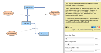
Once again we'll need to talk about differential equations:
- An SIR is a system of differential equations
(three of them, to be precise):
The simplest looks like this:
\[ \frac{dS}{dt} = -\alpha S I\\ \frac{dI}{dt} = \alpha S I - \beta I\\ \frac{dR}{dt} = \beta I \]
This simple SIR model generally assumes that
- The disease is short-lived and non-fatal.
- The disease is spread by contact between individuals.
- The individuals who recover develop immunity.
My Insightmaker
model includes the added possibility that the recovered population loses
immunity, so we'll eventually consider the system \[ \frac{dS}{dt}
= -\alpha S I + \gamma R\\ \frac{dI}{dt} = \alpha S I - \beta I\\ \frac{dR}{dt} = \beta I - \gamma R \]
But for most of this lab, you'll be taking $\gamma=0$.
These equations give the rates of change of the three populations. But, since the total never changes (no death), we just reshuffle the populations each time; and we must have a constant total population $N(t)=S(t)+I(t)+R(t)$.
- From calculus: What is $\frac{dN}{dt}$?
Write down everything you can about the derivative $\frac{dN}{dt}$.
- $\frac{dN}{dt}=0$, since it’s
constant. It’s also the sum of the three derivatives:
- $\frac{dN}{dt}=$\frac{dS}{dt}+\frac{dI}{dt}+\frac{dR}{dt}$
- Since $N=S(t)+I(t)+R(t)$
is some constant, we can write one of the populations in terms of the
others: e.g. $N-S(t)+I(t)=R(t)$.
- The terms on the right-hand side
of the system of differential equations, \[ \frac{dS}{dt} = -\alpha S I + \gamma R\\ \frac{dI}{dt} = \alpha S I -
\beta I\\ \frac{dR}{dt} = \beta I - \gamma R \] represent two
qualitatively different kinds of processes (and notice that everything
goes somewhere). The term $-\beta I\\$ is sort of a "death
term" of the infected: they die into the "new birth" of
the resurrection ($R(t)$ -- well, recovered!).
But the $\beta I$ term serves to increase the $R(t)$
population -- like a birth term.
Similarly, the $- \gamma R$ is like a death of the recovered, into a new life (birth) of a susceptible person. We think of it as a loss of immunity. Some vaccines wear off, and you need to be re-vaccinated: this is because you gradually lose your immunity.
The other type of term -- lost from the $S(t)$ population, but gained by the $I(t)$ population -- is an example of what we call "Mass-action dynamics": $\alpha S I$ represents a term that comes from the interaction of the $S$ and $I$ population. They have to collide -- come into contact -- to pass the infection from the $I$ to the $S$.
Check your initial settings:
|
$S(0)=S_0$ |
$60$ |
|
$I(0)=I_0$ |
|
|
$20$ |
|
|
$R(0)=R_0$ |
|
|
$20$ |
|
|
$\alpha$ |
|
|
$0.09$ |
|
|
$\beta$ |
|
|
$1.3$ |
|
|
$\gamma$ |
|
|
$0.0$ |
Notice that I've written the initial populations so that their sum, the total population, is 100. So we can interpret the populations as the percentage of the total population.
Notice also that you can set your rates with the sliders on the right, under the Insight information.
Set your time setting for months, 0 to 4; RK-4, with step-size of .1.
So here's the story:
- Experimentally it was determined that a certain
strain of flu spreading through this community satisfies the SIR model
with $a=0.09$ and $b = 1.3$. Initially there are 20% infected and there
are 60% who do not have, nor have ever had, this particular flu virus.
- Simulate and include your graph of populations
versus time.
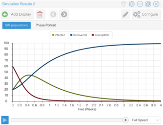
- Describe what's happened, in terms of the three
population as $t$ runs from 0 to 4 months. : The infected population rises to a peak, then there’s a
downturn, and an inflection point comes when it seems that the
infected population heads steadily to 0; while the number of susceptibles falls steadily toward an asymptote of 0; and
the number of recovered increases increasingly rapidly, then an
inflection point, and it begins to approach an asymptote of 100% of
the population. Everyone ultimately gets the virus, and everyone is
ultimately recovered, and immune.
- What happens as $t \to \infty$?
Why does this make sense? As
described above, the population is ultimately entirely recovered.
This makes sense, because as long as there are infecteds,
all the susceptibles will ultimately get
infected. Once infected, they’re bound to recover.
- Approximate the maximum fraction of the infected
population during first four months and when this occurs. At about .45 months, and about 45%
infected at the peak.
- Is the number of susceptibles
ever the same as the number of infected people when $0 \le t \le 4$?
If so, estimate when this occurs. Indicate where on the phase plot
this happens. At about time
t=0.2 months, and it would be where the phase portrait intersects the
line S=I.
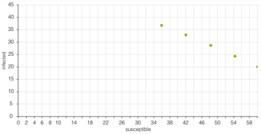
- Estimate the values of $S(2)$,
$I(2)$, and $I(3)$. These will be used in the next part. $S(2)=0.444$, $I(2)=8.681$, and $I(3)=2.440$
- From 1(d), you estimated $S(2),I(2),I(3)$.
Suppose that at $t = 2$ the flu virus mutates so that the value of $a$
is cut in half ($b$ remains the same at $b = 1.3$). So we need to restart the model,
but with $a$ half of what it was, but with $S(0)=0.444$,
$I(0)=8.681$, and awe want to find $I(1)$ to compare with what was $I(3)=2.440$.
- Use your Insightmaker
model to estimate $I$, the number of infected, 1 month after the virus
mutates. $I(1)=2.408$
- Compare this to the value of $I(3)$
from above. Explain the difference. So $I(1)$ is a fraction of what it
was -- $\frac{2.408}{2.440}$ -- but it’s a
pretty large fraction. It wasn’t cut in half, as $a$ was. Surprisingly
little change.
- Local officials will consider various strains of flu
an epidemic when the number of infected
reaches a maximum. Using the Insightmaker
model with the values shown in the tables below, estimate the values of
$S$ at the time $t^*$ when the number of infected is a maximum (don't
submit plots):
|
a) $a=0.125,
b=3$: \[ \begin{array}{|c|c|c|} {S(0)} & {I(0)}
& {S(t^*)}\cr \hline
{60}&{40}&{23.7}\cr \hline
{60}&{22}&{22.4}\cr \hline
{60}&{10}&{23.5}\cr \hline
{40}&{60}&{25.3}\cr \hline
\end{array} \] |
b) $a=0.167,
b=3$: \[ \begin{array}{|c|c|c|} {S(0)} & {I(0)}
& {S(t^*)}\cr \hline
{60}&{40}&{18.8}\cr \hline
{60}&{22}&{18.7}\cr \hline
{60}&{10}&{18.2}\cr \hline
{40}&{60}&{18.7}\cr \hline
\end{array} \] |
- For the SIR system (with $\gamma=0$) explain why you
should expect $I$ to reach a maximum when $S(t^*)=\frac{b}{a}$. When
$S(t^*)=\frac{b}{a}$,
the rate of change of $I(t)$ will
be 0 – so the population of infecteds will
have peaked. As S slips below this point, the sign of $\frac{dI}{dt}$ will be negative, and the
population of infecteds will fall.
- An official in the local government made several
statements to the press (shown below) concerning the strain of flu
modeled in the SIR, with $a =0.09$ and $b = 1.3$. Your job is to use Insightmaker to determine whether her statements
are accurate:
- Statement #1: If initially half the population is
susceptible but only 10% of the population is infected, then there
will never be more than 15% of the population infected. False:
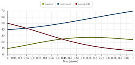
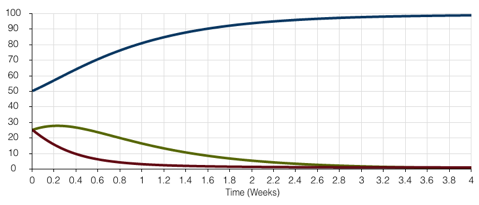
- Statement #2: If initially 25% of the population is
infected and 25% is susceptible, then the number of susceptibles is never again the same as the number
of infected. True (except in
the limit, as $t \to \infty$:
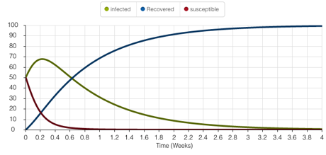
- Statement #3: If initially there are no individuals
with immunity and the number of susceptible and infected is the same,
then after 1 month at least 50% of the population will be in the
recovered group. True: about
70%:
(Include graphs to help support your claims about these statements.)
- Now (finally!) let's add some resusceptible
rate $\gamma$ into the mix. Set $\gamma=.02$,
$\alpha=0.008$, $\beta=0.41$, and $I(0)=1$ and $S(0)=99$.
Set the time to 144 months (twelve years), simulate and include your graphs, and answer these questions:
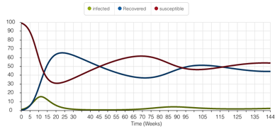
- Describe the course of the epidemic. Infected population takes off,
peaking at about 16% of the population after a year, as the susceptibles plummet, while the recovered
population soars. Then the epidemic goes quiet for a long while, and
then peaks again, about 90 months in (7.5 years down the road). It
looks like it will peak again, always less impactfully,
down the road (perhaps at about 14 years?).
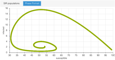
- What happens as $t \to \infty$?
(Does the phase portrait help you to decide?) The
population ends up with a steady state of susceptible, infected, and recovered
populations. The phase portrait
shows this by spiraling in on some fixed equilibrium values:
Links:
- Thanks to this
site for ideas.