- During class time I'll be on Zoom, at https://nku.zoom.us/j/7057440907.
Feel free to check in with questions or concerns.
- A reminder that the Math/Stat lab is now
on-line. Feel free to
- I hope that you're doing well, in spite of the difficulties.
- Today's Washington Post story A
negative coronavirus test result doesn't always mean you aren't
infected explains the dangers of Type I and Type II errors in
testing for Covid-19.
As they explain in the article, "Other tests may incorrectly say someone doesn't have a condition, but they do. That's a false negative, and for covid-19, the illness caused by the coronavirus, at this stage of the outbreak, experts are more worried about this type of inaccuracy."
In the context of a medical test, we test against a null of "no disease". If we reject a true null, we declare you diseased (when you're not) -- that's a type I error, and a "false positive".
What they're telling us is that they're worried more about false negatives, type II errors. So what we've learned in class is that they should relax their $\alpha$ for the hypothesis test. This makes it more likely to call you positive when you're not -- but also more likely to catch those who may test "negative" (and yet are positive, presumably infectious, and hence dangerous).
Key quote: "Everybody thinks the lab test is always right. When we design tests, they [often] have a 95 percent sensitivity, a 95 percent specificity. That means 5 percent of the time, you're wrong. That's just a structure of testing," Procop said. "You only want to test people you really do believe have the disease, and in this case, people you're going to act on. If it's an otherwise healthy, young person, you're going to say go home and isolate yourself."
- You have an Imath assignment due next Wednesday. Please keep up
with those.
- Last time I taught this course a student and I found a couple of
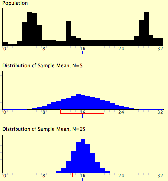
nice figure to explain what we're up to in this packet (I'll criticize
this first one at the end, but it's like a cartoon illustration):
We start with a wonky distribution for $y$ (top), really far from normal; with increasing sample size, the distribution of $\overline{y}$ will become more normally distributed, and as $n$ increases, more and more normal, with smaller spread.

Now for my criticism: that distribution at top is so wonky that $n=5$ wouldn't have healed it that well -- that $N=5$ distribution looks too normal. The spread is about right, because even an $n$ of 4 will cut the standard deviation in half -- and from the figure it seems that the N=5 distribution has cut its standard deviation to around 4, from the original 8 suggested by the bracket along the $x$-axis.
And the spread for the final $N=25$ distribution should be about a fifth ($\frac{\sigma}{\sqrt{25}}=\frac{\sigma}{5}$) of the original standard distribution, or about 8/5=1.6 units.
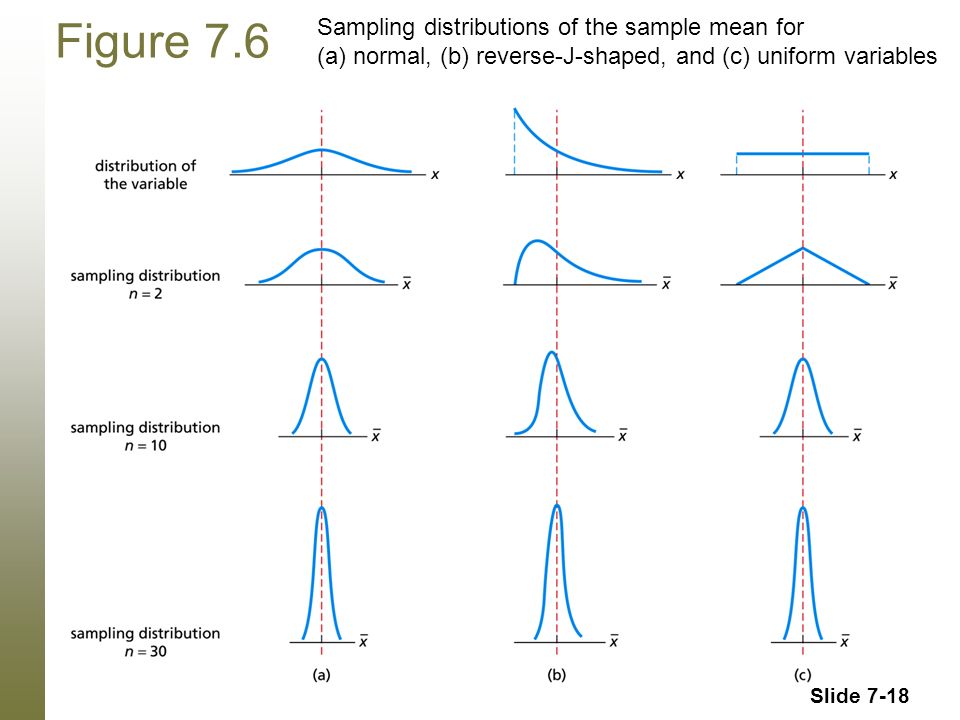
In the case of the skew distribution, it looks like even $n=30$ doesn't quite protect us: the distribution still has a "shrug" to it. Here we have three versions of the graph above, with more realistic results, for $n=2$, $n=30$, and $n=30$.

- With that as a reminder of what we're doing in this packet, let's
get back to Packet 8: Sampling Distribution
of the Sample Mean.
Sorry about the horrible audio in the following. This will improve, as I'm seeing using an iPad for recording.
I've prepared a video summary of the final filled-in packet, if you can't stand to go through the intro and examples with me....
- The Standard Normal Table of probabilities.
- Computing chi-squares in Statcrunch is carried out using the
Stat -> Tables -> Contingency ->
(then either data or summary, depending on what you have)