Tutorial to help you solve this problem
P(t) is the population size
at time t (measured in days)
P0 is the initial population size
K is the carrying capacity of the environment
r is a constant representing population growth or decay
Given all of your observations in the previous problems, and using the logistic model,
without any specific parameter values, explain what happens to the population size when r > 0 and t → ∞.
Do the same thing when r = 0 and r < 0 and t → ∞.
Tutorial
We are interested in knowing what happens to the population size P as t → ∞.
This of course depends on whether r is positive, negative, or zero.
Let's begin with r > 0. The logistic model (1), has only one
term that depends on t,
![]()
Thus, we conclude when r > 0 (i.e. birth rate > death rate t → ∞ implies P → K (i.e. the population approaches the carrying capacity.
Now let's consider the special case r = 0 (i.e. birth rate = death rate). If r = 0, the term in (2) reduces to K - P0, and there is no t dependence. Substituting this value into (1) gives,
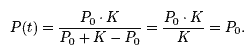
That is, if r = 0, the population size (at any time t) remains at the initial size, P0. This makes intuitive sense because r= 0 indicates that births are balancing deaths exactly.
Finally, let's consider the case r < 0. I r < 0, the term in (2) represents exponential growth. That is, t → ∞ implies (K - P0) · e-rt . → ∞. Since (2) is in the denominator of (1), we find that as t → ∞ ,
That is, the denominator in (1) becomes arbitrarily large as t → ∞ , resulting in P(t) → 0.
This makes sense when the death rate is larger than the birth rate.
*****