Problems

For each of the following functions, express the function in terms of operations on simpler functions.

1.   `ftext[(]x text[)]=x^3-4x^2`		2.  `gtext[(]x text[)]=-x^3+4x^2`
3.   `htext[(]x text[)]=|x^3-4x^2|`		4.  `jtext[(]x text[)]=sqrt(x^3+4x^2)`
5.   `phitext[(]t text[)]=t^(3//2)`		6.   `psitext[(]t text[)]=|t^(3//2)|`
7.   `lambdatext[(]t text[)]=|t|^(3//2)`		8.   `mutext[(]t text[)]=|t|^(-3//2)`

For each of the following functions, graph the function along with the simpler functions that were your answer to the corresponding Problem 1–8. (Note: The graphing calculator for Problems 9-12 requires `x` as independent variable, and the one for Problems 13-16 requires `t`.)

9.    `ftext[(]x text[)]=x^3-4x^2`		10.  `gtext[(]x text[)]=-x^3+4x^2`
11.   `htext[(]x text[)]=|x^3-4x^2|`		12.  `jtext[(]x text[)]=sqrt(x^3+4x^2)`
13.   `phitext[(]t text[)]=t^(3//2)`		14.   `psitext[(]t text[)]=|t^(3//2)|`
15.   `lambdatext[(]t text[)]=|t|^(3//2)`		16.   `mutext[(]t text[)]=|t|^(-3//2)`

You may need graph paper for the next several problems. Click on the image at the right to open a page from which you can print your own graph paper. Start each problem by labeling and scaling your axes in a way that is reasonable for that problem.

17. The data in Table P1 were collected by chemistry students who varied the temperature of a gas in a closed container and recorded the pressure exerted by the gas.
    
    

    Table P1   Temperature and pressure of a gas in a closed container

    Temperature (°K)	263	268	278	293	298	303	308	318	323
    Pressure (mm Hg)	752	755	777	811	834	840	854	892	906

    
    
    
    1. Make a scatter plot of the data in Table P1.
    2. When volume is held constant, is pressure related linearly to temperature? If so, how do you interpret the slope and `y`-intercept of the line?
    3. What change in pressure is brought about by a one-degree change in temperature?
    4. What change in temperature would cause a one-millimeter change in pressure?

 

18. Table P2   Highway deaths
    and miles driven
    (Source: NHTSA)

    Year	Deaths	Miles Driven (billions)
    1988	47,087	2,026
    1989	45,582	2,107
    1990	44,599	2,148
    1991	41,508	2,172
    1992	39,250	2,240
    1993	40,150	2,297
    1994	40,716	2,360
    1995	41,817	2,423
    1996	42,065	2,486
    1997	42,013	2,560
    1998	41,501	2,618
    1999	41,717	2,691
    2000	41,945	2,750
    2001	42,196	2,781
    2002	42,815	2,830
    2003	42,884	2,891
    2004	42,636	2,923

    Table P2 shows numbers of highway fatalities and billions of miles driven in the US from 1988 to 2004.
    
    
    1. Let `Dtext[(]t text[)]` and `Mtext[(]t text[)]` be the functions whose values are given in the second and third columns of Table P2, each as a function of time represented by the first column. Plot the functions `D` and `M` on separate coordinate systems.
    2. Let `Rtext[(]t text[)]` (for "rate") stand for the number of deaths per billion miles. How is `Rtext[(]t text[)]` related to `Dtext[(]t text[)]` and `Mtext[(]t text[)]`?
    3. Make a table for `Rtext[(]t text[)]` and plot the data in your table. What conclusions do you draw?
    4. Make up another question that can be answered from these data, and answer it.
    5. NHTSA reports numbers of deaths per hundred million miles, as in the following statement:

       "The fatality rate per 100 million vehicle miles traveled was 1.46 in 2004, down from 1.48 in 2003. The fatality rate has been steadily improving since 1966 when 50,894 people died and the rate was 5.5."

       How is NHTSA's rate related to your `Rtext[(]t text[)]`?

 

19. Table P3  Passenger car
    deaths and miles driven
    (Source: BTS)

    Year	Deaths	Miles Driven (billions)
    1990	24,092	1,427
    1991	22,385	1,412
    1992	21,387	1,436
    1993	21,566	1,445
    1994	21,997	1,459
    1995	22,423	1,478
    1996	22,505	1,499
    1997	22,199	1,528
    1998	21,194	1,556
    1999	20,862	1,567
    2000	20,699	1,580
    2001	20,320	1,593
    2002	20,569	1,608
    2003	19,460	1,608

    Table P3 shows numbers of highway fatalities and billions of miles driven in passenger cars in the US from 1990 to 2003.
    
    
    1. Let `Dtext[(]t text[)]` and `Mtext[(]t text[)]` be the functions whose values are given in the second and third columns of Table P3, each as a function of time represented by the first column. Plot the functions `D` and `M` on separate coordinate systems.
    2. Let `Rtext[(]t text[)]` (for "rate") stand for the number of deaths per billion miles. How is `Rtext[(]t text[)]` related to `Dtext[(]t text[)]` and `Mtext[(]t text[)]`?
    3. Make a table for `Rtext[(]t text[)]` and plot the data in your table. What conclusions do you draw?
    4. Make up another question that can be answered from these data, and answer it.
    5. (If you did the preceding problem) The passenger car data in Table P3 are included in the overall highway fatality data (all vehicles) in Table P2. Would you conclude that your chance of dying in a car on the highway is greater, less, or about the same as your chance of dying in any other kind of vehicle? Explain.
20. In Figure P1, is the function represented by the red data points the sum of the other three functions? Explain.

    
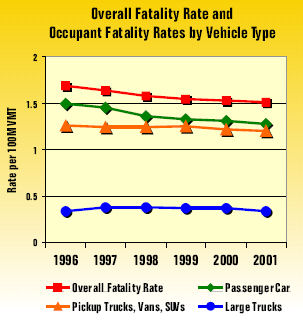
    Figure P1   Highway fatalities
    Source: NHTSA

21. Table P4 shows the dollar amounts of exports to and imports from Mexico over the period 1987 to 1996. Construct a table for the trade balance function, and graph this function.
    
    

    Table P4  Imports from Mexico to the United States
    Source: R. H. Ojeda et al., "North American Integration
    Three Years After NAFTA," UCLA, 1996

    Year	1987	1988	1989	1990	1991	1992	1993	1994	1995	1996
    Exports (billion dollars)	20.49	20.55	22.84	26.84	42.69	46.20	51.89	60.88	79.54	90.94
    Imports (billion dollars)	13.31	20.27	25.44	31.27	49.97	62.13	65.37	79.35	72.45	82.68

22. Figure P2 shows scatter plots of revenues and expenses for the Federal Employees Health Benefits (FEHB) program for fiscal years 1984 to 1996, both in billions of dollars.
    1. What would you call the difference of these two functions, revenue minus expenses?
    2. Tabulate and plot the difference function. What conclusions do you draw?
    
    Figure P2  Federal Employees Health Benefits Program Financial Data
    Source: US Office of Personnel Management 1998 Fact Book

23. Table P5   Values of a function

    x	0	1	3	6	8
    f(x)	0	2	3	4	5

    Some of the values of a function `f` are given in Table P5. Sketch a graph of the inverse of the function .
    
24. Show that the inverse of any linear function of the form `y=m x+b` (with `m\ne0`) is a linear function whose slope is `1text[/]m`.
25. 
    Figure P3   Graph of f(x)=x^2/3+3
    Does a linear function with slope `0` have an inverse? Why or why not?
26. The function f ( x ) = x 2 / 3 + 3 , x ≥ 0 , is graphed in Figure P3. Click on the graph to get a pop-up version of the same graph, and print the pop-up file. Then sketch a graph of the inverse function on the same axes.

     

     

    
    

Figure P4  Graph of f(x)=x3/8+x

The function `ftext[(]x text[)]=x^3 text[/]8+x` is graphed in Figure P4. Click on the graph to get a pop-up version of the same graph, and print the pop-up file. Then sketch a graph of the inverse function on the same axes. If `ftext[(]x text[)]=x^3 text[/]8+x`, make a table of values for `f^(-1)` with at least five entries. What's the problem with finding a formula for `f^(-1)` in this case?

Figure P5   Graph of a function f(x)

29. Figure P5 shows the graph of a function. Click on the graph to get a pop-up version of the same graph, and print the pop-up file. Then sketch a graph of the inverse function on the same axes.
30. 1. For the function `ftext[(]x text[)]` whose graph is shown in Figure P5, make a table of values for `f^(-1)` with at least five entries.
    2. What's the problem with finding a formula for `f^(-1)` in this case?

 


Figure P6   Graph of a function f(x)
31. Since “base 10 logarithm” is defined as the inverse of “base 10 exponentiation,” it may be that “base 10 exponentiation” is an answer to the question in Problem 14 of Section 1.4 about functions that turn sums into products. Show that this is true. [Hint: Recall what you have learned about properties of exponents.]
32. Figure P6 shows the graph of a function. Decide whether or not this function has an inverse, and give a reason for your answer.
33. The function graphed in Figure P6 has what kind of symmetry — even, odd, or neither? Give a reason for your answer.