Chapter 10
Polynomial and Series Representations of Functions
10.4 More Taylor Polynomials and Series
10.4.2 Taylor Polynomials and Series for `ln text[(]1 + xtext[)]`
We can use our knowledge of the Taylor polynomials for `1text[/(]1-xtext[)]` to obtain the Taylor polynomials for other functions. For example, since
we can substitute `x = -t` in the geometric series to find
We know from the more important part of the Fundamental Theorem that
What happens if we integrate the Taylor polynomials for `f text[(] t text[)] = 1text[/(]1+t text[)]`? We find
and, in general,
You will probably not be surprised to learn that
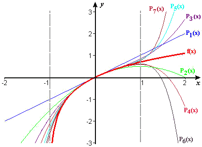
On the other hand, if `text[|] x text[|] > 1`, the polynomials in Checkpoint 1 do not approximate `ln text[(] 1 + x text[)]`. We can see this in Figure 1, which shows `f text[(] x text[)] = ln text[(] 1 + x text[)]` and its first seven approximating polynomials on the interval `[-2,2]`. As `x` approaches `-1` from the right, `f text[(] x text[)]` runs away to `-oo`. The successive polynomials `P_n text[(] x text[)]` all continue across the line `x = -1`, where there are no values of `f` to approximate. As `x` approaches `1` from the left, we see the successive polynomials getting closer to `f` at each `x` less than `1.` Then, as the curves cross `x = 1`, the higher degree polynomials run away from `f` faster than the lower degree ones.

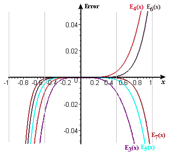
In Figure 2 we show the errors in the polynomial approximations plotted in Figure 1, again on an exaggerated scale. These low-degree polynomials have errors close to zero (i.e., fit well) only within about `1`/`2` unit of the origin. To get a good fit closer to `x=1` or `x=-1`, much higher degree polynomials are required.


