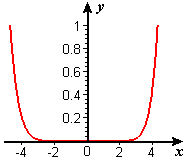
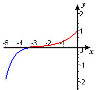
- We use two graphs, one for negative values of `x` and one for positive values, because the scales are so different. In both figures, the graph of `e^x` is in red and the graph of `P_9 text[(] x text[)]` is in blue. Figure C1 shows clear visual separation of `P_9 text[(] x text[)]` from `e^x` between `-3` and `-4`. In Figure C2, we don't see the separation until about `x=5`.
 |
 |
| Figure C1 Graphs of `e^x`
and `P_9 text[(] x text[)]` |
Figure C2 Graphs of `e^x`
and `P_9 text[(] x text[)]` |
-
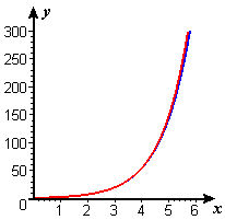
Figure C3 Graph of `e^x-P_9 text[(] x text[)]`
|
The graph of `e^x-P_9 text[(] x text[)]` in Figure C3 shows that the error is actually larger on the right. However, the error at `x=4` is less than 1% of the function value, and at `x=-4` it is many times the function value.
- The error is always positive. That is, `e^x>P_9 text[(] x text[)]` at every `x`.
For positive values of `x`, this is because the polynomial is the first 10 terms of a series for `e^x` in which all of the terms are positive. The tail also must be positive.
For negative values of `x` the explanation is harder, but eventually it is because the odd-degree polynomial must turn down and take negative values, whereas `e^x` never has negative values. This is why the separation is visually more evident on the left even though the error is larger on the right.