Chapter 2
Models of Growth: Rates of Change
 2.6
Logarithms and Representation of Data
Exercises
The data in each of the following tables (Exercises 1-4) approximately fit either an exponential function or a power function. In each case, decide which, and find a formula that fits the data. Each formula should have one of the forms `y=c b^t`, `y=c e^(k t)`, or `y=c t^k`, with explicit values for the constants.
| 1. | `t` |
`y` |
2. | `t` |
`y` |
||
|---|---|---|---|---|---|---|---|
0 |
0.0 |
0 |
2.709 |
||||
5 |
14.855 |
5 |
4.452 |
||||
10 |
20.292 |
10 |
7.339 |
||||
15 |
24.354 |
15 |
12.101 |
||||
20 |
27.720 |
20 |
19.950 |
||||
25 |
30.648 |
25 |
32.893 |
| 3. | `t` |
`y` |
4. | `t` |
`y` |
||
|---|---|---|---|---|---|---|---|
1 |
24.7 |
1 |
25.0 |
||||
5 |
17.2 |
5 |
7.5 |
||||
10 |
11.0 |
10 |
4.4 |
||||
20 |
4.5 |
20 |
2.6 |
||||
35 |
1.2 |
35 |
1.7 |
||||
50 |
0.3 |
50 |
1.3 |
-
The data in Table E2 are graphed in Figures E1, E2, and E3, in Cartesian, semilog, and log-log plots, not necessarily in that order.
-
Decide whether the data come from a linear function, a power function, an exponential function, or none of these.
- Estimate `ftext[(]2 text[)]`.
- Estimate `f'text[(]2 text[)]`.
-
-
The data in Table E3 are graphed in Figures E4, E5, and E6, in Cartesian, semilog, and log-log plots, not necessarily in that order.
-
Decide whether the data come from a linear function, a power function, an exponential function, or none of these.
- Find a formula for `f` as a function of `t` .
-
-
Table E6 shows the population of Mexico for each of the years 1980 through 1986.Table E6 Population
of MexicoYear Population
(millions)198067.38198169.13198270.93198372.77198474.66198576.60198678.59
- Find an exponential function that approximately fits these data.
- By what percentage did the population grow each year?
- What does your formula predict for the population in 2005?
-
Table E8 shows the U.S. Census data for the Houston, Texas, primary statistical metropolitan area over a period of 130 years.Table E8 Houston
area populationYear Population 185018,632186035,441187048,986188071,316189086,2241900134,6001910185,6541920272,4751930455,5701940646,8691950947,50019601,430,39419701,999,31619802,905,344
- Show that the historic population data for Houston are approximated by an exponential function, and find a formula for the function.
- Find the doubling time for Houston's population.
- If the growth pattern had continued to the present, what would Houston's population have been in 2007? (Compare with the Greater Houston entry in Wikipedia.)
- What would it be in 2050?
|
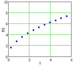 Figure E1 A plot of data in Table E2 |
||||||||||||||||||||||||
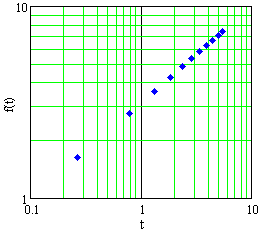 Figure E2 A plot of data in Table E2 |
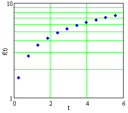 Figure E3 A plot of data in Table E2 |
|
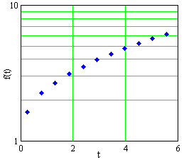 Figure E4 A plot of data in Table E3 |
||||||||||||||||||||||||
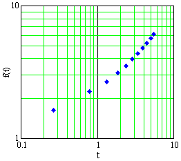 Figure E5 A plot of data in Table E3 |
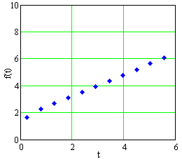 Figure E6 A plot of data in Table E3 |

