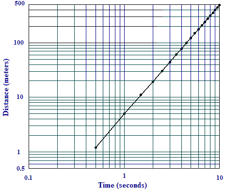
If we take the common logarithm, we find that `text(log) s=text(log) c+2 text(log) t text(.)` Since `text(log) c` is a constant, this equation has the form `y= text(constant)+2x`, where `y=text(log) s` and `x=text(log) t text(.)` Thus `text(log) s` is a linear function of `text(log) t` with slope `2 text(.)`
We can test this model by plotting `text(log) s` versus `text(log) t` to see if the points lie along a line of slope `2text(.)` In Figure A2, we show such a plot with both scales treated logarithmically, as we did with only the vertical scale in the semilog plots. This is called a log-log plot, or sometimes just a log plot.

The plotted points do seem to lie along a straight line. We can estimate the slope by checking the rise over the run for the extreme points:
Thus it looks like the model fits the data.