3.2.3 Solving the Initial Value Problem Symbolically

Now that we have seen a graphical interpretation of the solution of the initial value problem, we'll find a symbolic representation. Our differential equation for temperature of the cooling body is not exactly like the problems considered in Chapter 2 because the rate of change is proportional to $T-21$, not to $T$. That observation is what suggests the proposed change of dependent variable to $y=T-21$. Now

Thus, by substituting $y=T-21$ and $\frac{dy}{dt}=\frac{dT}{dt}$ into the original differential equation, we get a differential equation for the new unknown function `y`:

Also, at $t=0$, $T=30$, so $y=T-21=9$, which gives us an initial condition for the unknown function `y`. Thus, the substitution $y=T-21$ transforms the original initial value problem to a new initial value problem:

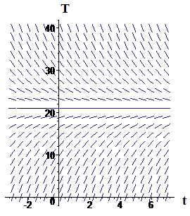
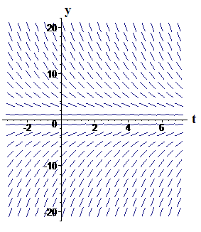
We illustrate the transformation from `T` to `y` in Figures 1 and 2. Figure 1 shows a slope field for the original differential equation. In Figure 2 we show the effect of the change of dependent variable, $y=T-21$, which is to move the horizontal axis from $T=0$ to the level of room temperature, $T=21$ or $y=0$. None of the slopes change because, at each value of `t`, $\frac{dy}{dt}=\frac{dT}{dt}$. Notice that the point `text[(]0,9text[)]` in Figure 2 corresponds to the point `text[(]0,30text[)]` in Figure 1.

Our new initial value problem,

should look familiar: It's the natural growth equation — except our growth factor is negative. The problem has exactly the form we saw in Chapter 2,

with $r=-k$. (In form, it is also the problem you studied in Activity 2, Activity 4, and Example 3 in the preceding section.) So the solution must have the form we saw in Chapter 2:

That is

Of course, `y` is not the quantity we wanted to know about — it was merely a computational convenience. But we can reverse the change of the dependent variable by substituting ${\displaystyle y=T-21}$ and solving for `T`:

Checkpoint 2