 |
 |
|
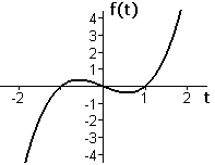
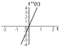
| Figure A1 Graph of `ftext[(] t text[)]=t^3-t` | Figure A2 Graph of `f''text[(] t text[)]=6t` |
Your graphs in part (a) should combine our Figures A1 and A2. The second derivative `f''` measures the rate of change of `f'`, that is, the rate of change of slope. The slope of the function `f` is decreasing when `t` is negative and increasing when `t` is positive.
 |
 |
|
| Figure A1 Graph of `ftext[(] t text[)]=t^3-t` | Figure A2 Graph of `f''text[(] t text[)]=6t` |
If you imagine walking along the graph of f from left to right, decreasing slope means you are turning right, and increasing slope means you are turning left. We describe the graph in the first case as concave down and in the second case as concave up. Thus, our function `ftext[(] t text[)]=t^3-t` has a graph that is concave down for negative values of `t` and concave up for positive values of `t`. As you trace out the graph with your finger, you should find that you have to shift the direction of the heel of your hand when the concavity changes
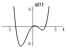
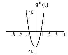
Figures A3 and A4 show graphs of `g` and its second derivative.
 |
 |
|
| Figure A3 Graph of `gtext[(] t text[)]=t^4-4t^2+2t` | Figure A4 Graph of `g''text[(] t text[)]=12t^2-8` |
The second derivative of `g` is positive for `t<-sqrt(2text[/]3)`, negative for `-sqrt(2text[/]3)<t<sqrt(2text[/]3)`, and positive again for `sqrt(2text[/]3)<t`. Thus, the graph of `g` is concave up for `t<-sqrt(2text[/]3)`, concave down for `-sqrt(2text[/]3)<t<sqrt(2text[/]3)`, and concave up again for `sqrt(2text[/]3)<t`.