4.3.1 Local Linearity

We have seen that analysis of the graph of a function leads naturally to the problem of finding zeros. This is the same problem as finding roots or solutions of equations in one variable — not a hard problem if you have a calculator with a Root or Solve key, or a computer algebra system, all of which have this functionality. In this section we explore how some of the basic ideas of differential calculus lead to an algorithm that could, in principle, be what's programmed into your calculator or computer. In reality, modern tools use somewhat more sophisticated ideas, but those are developed on the foundation of the basic ideas we discuss here. We will use the generic term "graphing tool" to refer to either a graphing calculator or a computer algebra system, whichever is convenient for you.

Activity 1

1. Use your graphing tool to graph the function `f` defined by

   ${\displaystyle f\left(t\right)=e^{3t}-t^2\mathrm{.}}$

2. Zoom in on the root near $-0.5\mathrm{.}$

3. Find numbers `b` and `c` such that you are sure  $b<$ root $<c$  and that the distance between `b` and `c` is less than $\mathrm{0.01.}$

4. Use the Root or Solve procedure on your graphing tool to find an approximation to the root that is accurate to `10` significant digits.

Comment on Activity 1

How did our computational tool find a 10-decimal-place solution of a nonlinear equation? (If you think that's not an interesting question, consider this: Somebody studying this text — maybe you — could turn out to be an electronic engineer designing the next generation of calculators or computer algebra systems. Even if that's not your goal, you should know something about how your tools work.) Figure A2 in the Comment on Activity 1 suggests an answer: A small segment of the graph — in particular, a segment close to the root — is nearly a straight line. That is, our nonlinear function is locally linear, so we can treat it like a linear function if the problem is sufficiently local.

Definitions   An equation in one unknown t is linear if it can be put in the linear form $mt+b=0$, where m and b are constants. Similarly, a function f is linear if the rule determining its values can be put in the linear form $f\left(t\right)=mt+b$. An equation is nonlinear if it cannot be put in the linear form, and a function f is nonlinear if the rule determining its values cannot be put in the form $f\left(t\right)=mt+b$.

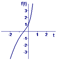
For example, the equation $3t+7=13$ is linear, since it can be put in the form $3t-6=0.$ Similarly, the function `f` defined by $f\left(t\right)=3t-6$ is linear. On the other hand, the equation $e^{3t}-t^2=0$ is not linear, and neither is the function `f` defined by ${f\left(t\right)=e}^{3t}-t^2\mathrm{.}$ The graph of a linear function is a straight line. The graph of a nonlinear function (see Figure 1) is something other than a straight line.

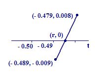
Here is one possibility for what our computational tool did in Activity 1. We identified the points $(-0.489,-0.009)$ and $(-0.479,0.008)$ on the graph of `f` when we entered lower and upper bounds. These points are close to — and bracket — the point $(r,0)$ where the graph of `f` crosses the `t`-axis. If the segment of the graph connecting these bounding points is sufficiently linear, then we can locate $(r,0)$ as a point on the line segment connecting the bounding points — see Figure 2.

The slope of the line segment can be calculated in two ways as "rise over run." First we calculate the slope using the upper right point, $(-0.479,0.008)$ and the lower left point, $(-0.489,-0.009)$:

Now we calculate the slope using the upper right point $(-0.479,0.008)$ and the point of intersection with the `t`-axis $(r,0)$:

Since these two calculations of the slope must be the same, we may set them equal:

When we clear the fraction and solve for `r` (check the details), we get

That's the right answer to `3` decimal places — the error is about `0.0002` — but not to `10` places.

In principle, our calculator could repeat the process, using $-0.48370$ as the next guess. However, we are going to look next at a slight variation of this idea. Instead of using the slope of the line segment connecting two bracketing points, we will use the slope at our current guess, calculated as a value of the derivative.