Chapter 4
Differential Calculus and Its Uses
4.5 The Chain Rule
4.5.4 Analysis of Reflection
With the necessary differentiation tools in hand, we return to our investigation of the reflection of light. In Figure 3, we have labeled the object `P`, the viewer's eye `Q`, and the image `R` of the object in the mirror. For fixed positions of the mirror, the object being viewed, and the eye, the quantities that are constant are the distance `p` from object to mirror, the distance `q` from eye to mirror, and the distance `D` between the projections of object and eye on the mirror. In principle, until we know the relationship between `alpha` and `beta`, the point `R` could be anywhere along the mirror. We label its distance from the left edge of the figure by `x`, and we imagine that `x` can take any value from `0` to `D`. Our question, then, is what value of `x` produces the minimal travel time for a ray from `P` to `R` to `Q`? When we can answer that question, we will know how `alpha` and `beta` are related.
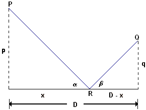
Figure 3 Reflection of a light ray in a mirror
Since the speed of light in air is constant, minimizing the time-of-travel for the light ray is equivalent to minimizing the distance traveled, i.e., the sum of the distances from `P` to `R` and from `R` to `Q`. Both distances depend on `x`, of course, so their sum does also.
Activity 3
-
Figure 3 contains two triangles. We have explained the labeling of three of the six sides. Explain the fourth distance label, `D-x`, in the figure.
Calculate the lengths of the two remaining sides, and label them accordingly.
Find a formula for the length of path function `Ltext[(]xtext[)]` for any `x` between `0` and `D`.

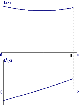 |
| Figure 4 L(x) and its derivative |
Figure 4 also has a message about the limitations of graphical and numerical methods for solving the type of problem we are studying now. First, in order to draw the graph of `L`, we had to specify values of the constants `p`, `q`, and `D`. If we made different choices, would the graph look the same? We want to know the relationship between `alpha` and `beta` regardless of the values of the constants.
Second, as we observed in Section 4.1, we would have a problem finding the leveling-off point on the graph of `L` by zooming in on it. That portion of the graph is already very flat, and when we zoom in we will see nothing but a horizontal line long before the scale is fine enough to tell us anything about the lowest point. We could zoom in instead on the graph of `L'` to find where it crosses the `x`-axis but only if we know a formula for `L'`, or at least some way to compute its values. Similarly, we could apply Newton's method to the equation `L'text[(]xtext[)]=0`, but for that we need to be able to compute values of both `L'` and its derivative, `L''`. Thus, even with graphical and numerical tools at hand, we still have to come to grips with the problem of calculating `L'`.
Activity 4
Calculate
`d/(dx)[q^2+text[(]D-xtext[)]^2]`
`d/(dx)sqrt(q^2+text[(]D-xtext[)]^2)`
`d/(dx)Ltext[(]xtext[)]`
Notice what happened here: From two very simple formulas the Power Rule and the Chain Rule the first very specific, and the second very general, we differentiated a very complicated formula, one we could never have dealt with directly by using difference quotients. Now what did we learn about reflection? Well, `L'text[(]xtext[)]=0` is equivalent to
That still looks like a substantial algebraic challenge, but let's keep our goal in focus. We wanted to determine the relationship between `alpha` and `beta`, and the two quotients in the above equation have a direct connection with those two angles. In Figure 3, we see that each numerator in the equation is the length of an adjacent side for one of the angles, and each denominator is the length of the corresponding hypotenuse. Thus, the equation reduces to a very simple statement about the angles:
And, as both angles are between 0° and 90°, the only way they can have the same cosine is to be the same angle. Conclusion:
That conclusion probably comes as no surprise to you. Indeed, you probably figured it out from our mirror experiment.