Chapter 4
Differential Calculus and Its Uses
4.8 Differentials and Leibniz Notation
4.8.2 Zooming In — Again
At most points on the graphs of most functions, a sufficiently small segment of the curve looks like a straight line, and the slope of that line is what we called the instantaneous slope of the function, i.e., the derivative. Figure 1 is like our zooming figures in Chapter 2, with these exceptions:
- The point at which we are doing the zooming is at the left edge of each picture, not in the center.
- We have added a line tangent to the graph at the left edge of the figure.
Move the mouse over the plot below to see a succession of plots of `y=t^2` zooming in on the point on the graph at `t=1`. Alternately, you may use your plotting tool to zoom in at any rate you please.
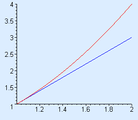
Figure 1 Zooming in on the graph of a smooth function
As we zoom in, the curve eventually appears to coincide with the tangent line. Indeed, the line whose slope we called the derivative is the tangent line at the point at which we are calculating instantaneous rate of change. What we conclude from this and similar activities is that, at any particular point on the graph of a smooth function `y=ytext[(]t text[)]`, the derivative `dytext[/]dt` is the slope of the tangent line at that point.
As a slope, `(dy)/(dt)` is also a rise over run. What rise, and what run? Since the tangent line is a line, we can take any run we like and calculate the corresponding rise — the ratio of rise to run is constant. Suppose we name the run `dt` (even though it already has the name `Delta t`) and the rise `dy`. Then we will have identified two quantities, `dy` and `dt`, whose ratio is indeed the derivative. That's it!
| Definitions The differential of `t`, calculated at a particular point on the graph of `y=y(t)`, is a (possibly small) change in `t`, and the differential of `y` is a corresponding change in `y` not on the graph of `y=y(t)`, but on the tangent line at the point in question. |
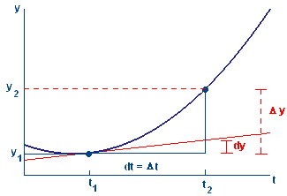
Figure 2 Rise to the curve (`Delta y`) and rise to the tangent line (`dy`) for a given run `Delta t` (or `dt`)
| `Delta y` is the rise to the curve after a run of `Delta t.` |
| `dy` is the rise to the tangent line after a run of `dt.` |
When we take `dt` and `Delta t` to be the same run, `Delta y` and `dy` are clearly different, and it follows that the slopes `(Delta y)/(Delta t)` (between two points on the curve) and `(dy)/(dt)` (between two points on the tangent line) are also different.
However, we know the figure is an exaggeration. Our zoom-in figures show what happens when we consider a very small run: The rise to the curve and the rise to the tangent line are approximately equal. In one sense, we already knew that. We introduced the derivative as the limiting value of difference quotients (slopes between points on the curve) when the run shrinks to zero. Thus, for a very small run, the slope between points is approximately the slope at a point, i.e., the derivative. If the slopes are approximately equal, the rises also must be.
In another sense, we have a new idea in the approximate equality of the two rises:
This says that we can approximate an actual change in values — a rise on the curve — by something that may be easier to compute, a rise on a straight line. Indeed, for the line, if we know the slope and the run, then we know the rise. The idea is not entirely new — we used this concept in Section 4.4 to derive the Product Rule.