6.2.1 Natural Versus Constrained Growth

In Chapter 2 we examined simulated fruit fly data and concluded (from a semilog plot) that the growth was natural (i.e., exponential). We modeled the growth by the differential equation

and, as we saw in Chapter 2, the solutions of this equation are of the form

Natural growth occurs for relatively short periods of time in settings from lab colonies of fruit flies to the population of Houston, Texas. However, this type of growth cannot continue indefinitely -- otherwise, the world would fill up with flies or Texans.

A somewhat more realistic model for biological growth, where resources are constrained by the environment, is the logistic model, whose differential equation is

where `k` is a positive proportionality constant and `M` is the maximum population that the environment can support.

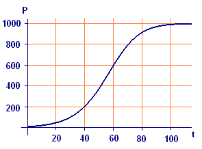
In Figure 1 we show a numerical solution to the logistic equation for `k=0.00009,` `M=1,000,` and `P_0=10.` This S-shaped curve is called a logistic curve.

Activity 1

Use your computer algebra system to display the Euler's Method solution for the logistic equation initial value problem represented by Figure 1.

1. How does the solution change as `M` is varied?

2. How does the solution change as `k` is increased? decreased?

3. How does the solution change as `P_0` is increased, but remains less than `M?`

4. How does the solution change if `P_0` is increased to a value greater than `M?`

5. What can you say about the solution if `P_0=M?`

Comment on Activity 1

In the next activity you will use the differential equation itself to explain the behavior of the solutions that you observed in Activity 1.

Activity 2

1. How does the factor `M-P` affect the growth rate of the population when `P` is small relative to `M`?

2. How does the factor `M-P` affect the growth rate when `P` is close in value to `M`?

3. How does the factor `M-P` affect the growth rate when `P` is greater than `M`?

Comment on Activity 2

As with any differential equation, the constrained growth model

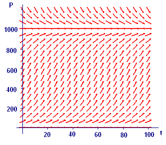
has infinitely many solutions -- Figure 2 shows the corresponding slope field. The complete model for constrained growth is an initial value problem consisting of the differential equation and an initial condition,

That is, we assume we know the population at some particular time, which we then designate time zero. Our fundamental assumption is that any initial value problem has a unique solution. Thus, once we have found any solution at all, it must be the only one.

Activity 3

Use your computer algebra system to display the slope field shown in Figure 2.

1. Display on the slope field the unique Euler's Method solution to the corresponding initial value with `Ptext[(]0text[)]=10`.

2. Display on the slope field the unique Euler's Method solution to the initial value problem with `Ptext[(]0text[)]=111`. The first part of this solution should be a reasonable model for the fruit fly data.

3. Add a few more solutions with starting points of your own choosing.