6.3.6 Testing for Logistic Growth

In Chapter 2 we introduced logarithmic plotting as a tool for deciding whether data on a growth pattern might fit either an exponential model or a power model. Here we explore a similar idea for deciding whether data points might fit a logistic model — and, if so, to determine the parameters in the model.

One of our steps in using antidifferentiation to find a symbolic solution of the differential equation

d ⁢ P d ⁢ t = k ⁢ P ⁢ ( M - P )

was the equation

1 M ⁢ ln ⁢ P M - P ⁢ = k ⁢ t + C .

The right-hand side of this equation is a linear function of time `t`, and the left-hand side is a computable function of population `P` — if we know or can find a value for the maximum supportable population `M`. But that's a big IF.

Here are some possible strategies:

1. If the data appear to have leveled off, say, at `P=P`_final, then we can set `M=P`_final. This is very unlikely for any biological population, except in a tightly controlled environment.
2. Use the result of Exercise 9 in Section 4.5, which relates the maximum supportable population to the maximal growth rate, which in turn occurs at the inflection point of the data. This may not work unless the data are unusually "smooth", and it certainly won't work if the available data have not yet reached the inflection point.
3. Conduct computer experiments by varying `M` in your computation of the left-hand side until the results are as straight as possible.

We illustrate the use of the second and third strategies in the following Example.

Example: U. S. Population, 1790-1940

Table 1 shows the U. S. Census data for the entire 210 years that the census has existed. As we have noted, P. F. Verhulst was able to use only the first six data points to predict the population 100 years later. We will explore why the first 16 points are neatly fit by a logistic curve. In Figure 3, we show those first 16 points.

Table 1   U.S. Census Data for Total Population Date Population (millions)   Date Population (millions) 1790 3.929   1900 75.996 1800 5.308   1910 91.972 1810 7.240   1920 105.711 1820 9.638   1930 122.775 1830 12.866   1940 131.669 1840 17.069   1950 150.697 1850 23.192   1960 179.323 1860 31.443   1970 203.185 1870 38.558   1980 226.546 1880 50.156   1990 248.710 1890 62.948   2000 281.422

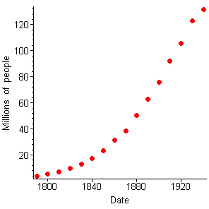Figure 3   U.S. Census Data for Total Population

Verhulst didn't have enough data to estimate the inflection point, but we do (and would have in 1940). It looks as though that point occurred around 1910, when the population would have been about 90 million, so a good guess at `M` would be 180 million. (Why? This is where the second strategy comes in.)

It is notoriously difficult to "see" an inflection point on a curve, let alone in a set of data points, with any accuracy. We could continue the example with any reasonable choice of `M` — to be candid, the number "180" is the result of having already used the third strategy, of trying plots with a computer algebra tool, and settling on that one as a good choice.

With the choice of `M=180`, we plot

1 M ⁢ ln ⁢ P M - P

against time `t` (normalized for convience so that `t=0` in 1790), and we get the nicely linear result shown in Figure 4. The data point for 1930 is a little out of line, but we could see already in Figure 3 that it was a little high for a curve that would pass smoothly through the other data points.

Figure 4   `1/M ln P/(M-P)` as a function of time in decades from 1790

For this time scale, it appears that the `y`-intercept `C` for the linear function `kt+C` is about `-0.021`. To find the slope `k`, we can choose any two points that we expect to be on the line, say the first and last. That slope turns out to be about `0.00178`. With those choices, we get the linear fit shown in Figure 5.

Figure 5   `1/180 ln P/(180-P)=0.00178 t-0.021`,
where `t` is time in decades from 1790

Now we come to the "acid test": We plot our computed formula (with `P_0=3.929`, the population in 1790) together with the actual census data (Figure 6).

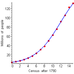
Figure 6  `P=(3.929 times 180)/[text[(]180-3.929text[)] e^(-180 times 0.00178 times t)+3.929]`

That's the end of our example showing how it was possible for Verhulst to predict the 1940 population — but of course we used information not available to him in 1840. Lest we get too cocky about the power of our predictive tools, here's the rest of the story: Figure 7 shows the remaining six censuses along with the continuation of our model function.

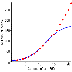
Figure 7   `P=(3.929 times 180)/[text[(]180-3.929text[)] e^(-180 times 0.00178 times t)+3.929]`

Checkpoint 5