Exercises

1. 1. What is the average value of the function `ftext[(]t text[)]=7` for `-2<=t<=3`? How do you know?
   2. What is the average value of a constant function `ftext[(]t text[)]=c` on the interval `[a,b]`? Explain.
2. 1. What is the average value of the function `ftext[(]t text[)]=2t` for `0<=t<=3?` How do you know?
   2. What is the average value of a linear function `ftext[(]t text[)]=ct` on the interval `[0,b]`? Explain.
3. 1. What is the average value of the function `ftext[(]t text[)]=2t+7` for `-2<=t<=3`? How do you know?
   2. What is the average value of a linear function `ftext[(]t text[)]=ct+p` on the interval `[a,b]`? Explain.
4. Calculate the exact value of each of the following integrals.

   `int_(-2)^3 7 dt`	`int_a^b c dt`
   `int_0^3 2t dt`	`int_0^b ct dt`
   `int_(-2)^3 (2t+7) dt`	`int_a^b (ct+p) dt`

5. Calculate each of the following sums.

   `sum_(k=1)^6 k`	`sum_(k=1)^6 (k-1)/2`
   `sum_(k=1)^6 2k`	`sum_(k=1)^6 (k+1)/2`
   `sum_(k=1)^6 k/2`	`sum_(k=1)^6 k^2/2`

6. Table E1   
   Values of
   an unknown
   function

   `t`	`ftext[(]t text[)]`
   0	0
   0.25	0.01618
   0.5	0.125
   0.75	0.39775
   1.0	0.86603
   1.25	1.50926
   1.5	2.25
   1.75	2.95815
   2.0	3.4641
   2.25	3.57973
   2.5	3.125
   2.75	1.95732
   3.0	0

   This exercise and the next concern a function `f` that is continuous on the interval `0<=t<=3`. Some values of `f` are given in Table E1. For each of the following values of `n`, calculate `sum_(k=1)^n ftext[(]t_(k-1) text[)] Delta t`, where `Delta t=3text[/]n`, and `t_k=k Delta t` for `k=0,1,...,n`.
   
   

   a.  `n=3`

   b.  `n=4`

   c.  `n=6`

   d.  `n=12`

7. For the function `f` whose values are given in Table E1, estimate
   
   
1. `int_0^3 ftext[(]t text[)] dt`
2. the average value of `f` on the interval `[0,3]`.
8. 1. Divide the interval `[0,1]` into four parts, and estimate `int_0^1 t^3 dt`.
   2. Divide the interval `[0,1]` into ten parts, and estimate `int_0^1 t^3 dt`.
   3. Make a guess at the exact value of `int_0^1 t^3 dt`.
9. Estimate the value of each of the following integrals.

   `int_0^2 sqrt(x) dx`	`int_0^0.8 x^4 dx`
   `int_0^1 x^(4//3) dx`	`int_0^pi sin x dx`
   `int_0^2 e^(-2x) dx`	`int_(-1)^1 (1-x^2) dx`

10. Estimate the average value of each of the following functions on the given interval.

    `sqrt(x), 0<=x<=2`	`x^4, 0<=x<=0.8`
    `x^(4//3), 0<=x<=1`	`sin x, 0<=x<=pi`
    `e^(-2x), 0<=x<=2`	`1-x^2, -1 <=x<=1`

11. Learn how to use the integral function of your computer algebra system or calculator, and use it to evaluate each of the following definite integrals. Use the results to check your estimates in Exercise 9.

    `int_0^2 sqrt(x) dx`	`int_0^0.8 x^4 dx`
    `int_0^1 x^(4//3) dx`	`int_0^pi sin x dx`
    `int_0^2 e^(-2x) dx`	`int_(-1)^1 (1-x^2) dx`

12. Find `int_a^b |x| dx`. Distinguish carefully the following cases:

    a.  `0<=a<=b`

    b.  `a<=b<=0`

    c.  `a<=0<=b`

13. Let `ftext[(]x text[)]=|x|^(1/3)`.
    1. Graph `ftext[(]x text[)]` on the interval `[-2,2]`.
    2. Explain why `f` is a continuous function.
    3. Estimate `int_(-2)^2 ftext[(]x text[)] dx`.
    4. Use your computer algebra system or calculator to evaluate `int_(-2)^2 ftext[(]x text[)] dx`.
14. In the discussion of Activity 1, we observed that the newspaper average temperature - the average of high and low - could be different from an average based on a modest number of sample points or from a continuous average.

    1. Sketch the graph of a continuous function whose average value must be quite different from the average of its high and low values on a given interval.
    2. Explain how you know that the two averages are different.
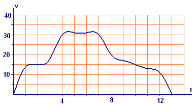
15. In all our calculations of distance traveled by the car (see Figure E1), we estimated the distance for a short time interval by multiplying the speed at the left endpoint (i.e., at the start of the interval) by the length of the interval. We could have just as well used the speed at the right endpoint of the interval.

    
    Figure E1  Speed `vtext[(]t text[)]` in MPH as a function of time `t` in minutes

    1. Show that for the speed function in Figure E1., the total distance estimates would be the same using either choice of constant speed for the subintervals. That is, show that

       `sum_(k=1)^n vtext[(]t_(k-1) text[)] Delta t = sum_(k=1)^n vtext[(]t_k text[)] Delta t`.

    2. What feature of this particular trip makes the preceding equation a true statement?
    3. Would you expect this equation to be true for every velocity function on every time interval? Why or why not?
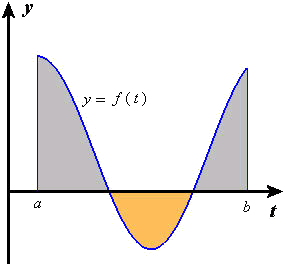
16. Suppose the values of a function `ftext[(]t text[)]` are positive for some values of `t` and negative for others, as in Figure E2. Think about how the negative values of `f` enter into the calculation of the definite integral and how they relate to areas of rectangles. What geometric interpretation can you give to the value `int_a^bftext[(]t text[)] dt`?

    
    Figure E2  How is `int_a^bftext[(]t text[)] dt` related to the shaded areas?

17. Suppose the function in Figure E2 represents the velocity of a moving object at time `t`. (Velocity is positive if the object is moving forward, negative if it is moving backward.)
    1. What physical interpretation can you give to the value `int_a^bftext[(]t text[)] dt`? Is your answer to this question consistent with your answer to Exercise 16?
    2. What would it mean if the value of the definite integral turned out to be zero? What would that mean in the geometric context of Exercise 16? What would that say about the average value of the function between `a` and `b`?

18. Table E2   Record of
    sample temperatures

    Time	Temperature
    12-5 AM	42°F
    5-7 AM	57°F
    7-9 AM	72°F
    9 AM - 1 PM	84°F
    1-4 PM	89°F
    4-7 PM	75°F
    7-9 PM	66°F
    9-12 PM	52°F

    To determine the average temperature for a day, a meteorologist decides to record the temperature at eight different times during the day. She further decides that these recordings do not have to be at equal time intervals, because she does not need several readings during times when the temperature is not changing very rapidly - and she doesn't want to get up in the middle of the night. Her data, shown in Table E2, include one reading in each of the time intervals shown. Use her data to estimate the average temperature for the day.

    Problem adapted from Calculus Problems for a New Century, edited by R. Fraga, MAA Notes no. 28, 1993.

19. 1. Find a region of the `xy`-plane whose area is given by the integral `int_0^1sqrt(1-x^2) dx`.
    2. Find the exact value of this integral.
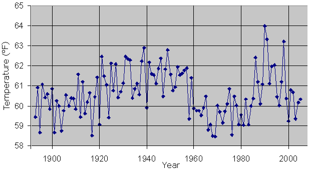
20. Figure E3 shows the annual average temperature in Charlotte, North Carolina for the period from 1893 through 2005.
    1. Estimate the average temperature in Charlotte for the period 1893-2005.
    2. Estimate the area under the data curve and above the time axis for the same period.

21. Our description of `int_a^bftext[(]t text[)] dt` for continuous functions works equally well for functions that can be described by a finite family of different continuous functions, one for each of a corresponding family of subintervals constituting `[a,b]`. Such functions are called piecewise continuous.
    1. Estimate the integral from `0` to `3` of the function `f` described by

    `ftext[(]t text[)]={(t^2,if 0<=t<=1),(t-1,if 1<t<=2), (sin t , if 2<t<=3):}`  .

    2. Use a graphing tool to graph this function. Check that your estimate in part (a) is consistent with the area under the graph of the function. [Hint: For some graphing tools, this function can be defined by a formula of the form

       `ftext[(]t text[)]=t^2 (0<=t) (t<=1)+(t-1) (1<t) (t<=2)+(sin t) (2<t) (t<=3)`.

       Each of the inequality expressions in parentheses has the value `1` if the inequality is satisfied and `0` if it is not.]
22. Among the piecewise continuous functions, in the sense of the preceding exercise, are the step functions, that is, functions that are constant on particular intervals but not necessarily over the whole domain. An example of such a function is the first-class postage function, `p=ftext[(]w text[)]`, where `w` is the weight of a letter in ounces, and `p` is the postage in cents. As of 2006, this function has the following values: For `0<w<=1`, `ptext[(]w text[)]=39`. For each additional ounce, add `24` cents. Find

    `int_0^5 ftext[(]w text[)] dw`.