7.1.2 Average Speed and Distance Traveled:
         First Estimate

We turn our attention now to a more familiar situation: your car's speedometer and odometer. We can only imagine that you have a continuous pen recorder for your speed, but speed has a distinct advantage over temperature because we already know an easy way to compute average speed for a trip — just divide total distance by total time. Whatever "average" means for a continuous function, it should give the same answer.

Activity 2

Suppose we attach a graphical recorder to the speedometer of your automobile, and on a `13`-minute trip between two red traffic lights, it records speed (as a function of time) as shown in Figure 3. Roughly how far apart are the two traffic lights?

Comment on Activity 2

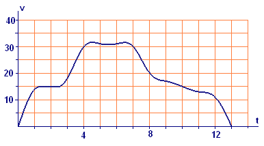
We will estimate the distance by dividing the time interval into `13` one-minute subintervals, estimating the distance traveled in each of these shorter intervals, and adding the estimates. The speeds at each minute mark are shown in Table 1. Since the minute is our unit of time, we have converted the speeds to miles per minute.

Checkpoint 1

In a single one-minute interval — except for the first and last—there is not much change in speed. Thus we can estimate the distance traveled in one minute by assuming that the speed is constant. If the speed is constant, then that speed is the average speed, and the distance traveled is that speed times the time.

Therefore, we estimate the distance traveled in a particular time interval, say, from `2` minutes to `3` minutes, by assuming that the speed is constant at `0.25` miles per minute for the whole minute. That is, we estimate the distance traveled between the `2`-minute mark and the `3`-minute mark to be

(Speed at `2` minutes)`times`(`1` minute)`=0.25 times 1=0.25` miles.

If we designate the speed function in miles per minute by `vtext[(]t text[)]`, then our estimate of the distance traveled in the time interval from `t=k-1` minutes to `t=k` minutes is `vtext[(]k-1 text[)] times 1 = vtext[(]k-1 text[)]` miles. Our estimate for the total distance is then the sum of these `13` estimates or

Distance`~~ vtext[(]0 text[)]+vtext[(]1 text[)]+vtext[(]2 text[)]+vtext[(]3 text[)]+ ... + vtext[(]11 text[)]+vtext[(]12 text[)]`.

This is just the sum of the numbers in the third column of Table 1 [because `vtext[(]13 text[)]=0`], so our estimate of the distance is `4.09` miles.

Checkpoint 2

Lengthy sums like

`vtext[(]0 text[)]+vtext[(]1 text[)]+vtext[(]2 text[)]+vtext[(]3 text[)]+ ... + vtext[(]11 text[)]+vtext[(]12 text[)]`

will turn up frequently in what follows. Even with only `13` terms, we didn't write all the terms explicitly. When we have sums with hundreds of terms, this wouldn't even be an option. Thus we will make a practice of writing sums in sigma notation. If you are unsure what sum is represented by a given sigma notation, you should write out explicitly at least the first few and the last few terms, as we did in our sum of table entries. Here is the same calculation expressed in sigma notation:

Distance ${\displaystyle \approx \sum _{k=1}^{13}v(k-1)}$

We read the right-hand side of this equation as "the sum of terms of the form `vtext[(]k-1 text[)]` where `k` runs from `1` to `13`." Can you see why that means the same thing as the long-hand sum at the start of this paragraph?