7.1.5 Area Under a Curve

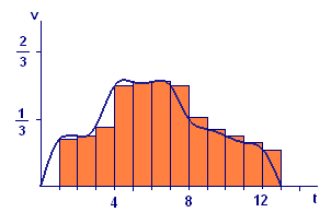
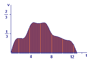
We prepare the way for the Fundamental Theorem by giving our distance estimates a geometric interpretation. Consider again the estimate of total distance obtained from the `13` one-minute subintervals. The estimate for distance traveled in the particular subinterval `[2,3]` is `vtext[(]2text[)] times 1`. This is the area of a rectangle with base from `t=2` to `t=3` and height `vtext[(]2text[)]`. In general, the estimate for distance traveled in the time interval `[k-1,k]` is the area of the rectangle with base from `t=k-1` to `t=k` and height `vtext[(]k-1text[)]`. When we superimpose these rectangles on the graph of `vtext[(]t text[)]`, we obtain part (i) of Figure 5.

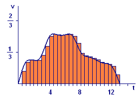
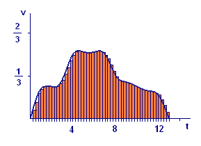
Our estimate using `n` equal subintervals of total distance traveled is the sum of the areas of `n` rectangles, the `k`th one with base from `t_(k-1)` to `t_k` and height `vtext[(]t_(k-1)text[)]`. We show the cases for `n=26`, `n=52`, and `n=104` in the remaining parts of Figure 5.

Figure 5   Geometric interpretation of successive estimates of distance

(i) `n=13`	(ii) `n=26`
(iii) `n=52`	(iv) `n=104`

It is apparent from Figure 5 that the number `4.12` toward which the estimates are tending is the area of the region bounded above by the curve `v=vtext[(]t text[)]` and below by the `t`-axis for `0 ≤ t ≤ 13`. Think of approximating the region by placing a large number of rectangular strips side by side. As the number of strips increases (and their widths decrease), the rectangular polygon formed by them fits the region bounded by the curve better and better. Thus the sum of the areas of the rectangles comes closer and closer to the area of the region under the curve.

There is nothing special about the particular speed function `vtext[(]t text[)]` in Figure 5 or about the particular time interval `[0,13]`. For an arbitrary continuous speed function `vtext[(]t text[)]` and an arbitrary time interval `a ≤ t ≤ b`, we can describe the distance traveled and its relationship to area in the following way:

The total distance traveled by an object moving with speed `vtext[(]t text[)]` from time `t=a` to time `t=b` is the limiting value (as `n` becomes large) of the sums

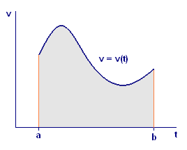
where `Delta t = text[(]b-atext[)/]n` and `t_k=a+k Delta t` for `k=0, 1, ... , n`. Moreover, this distance is also the area of the region in the `text[(]t,vtext[)]`-plane sketched in Figure 6.

Contents for Chapter 7