In the information age we are absolutely dependent on electronic devices all around us — computers, calculators, voice mail, fuel injectors in our cars, automatic teller machines, product scanners in checkout lines, and so on, not to mention iPods and MP3 players. These things have a way of wearing out or burning out at the most awkward times — for example, when your disk drive goes haywire and trashes the only copy of your term paper. We're going to study the question of component failure, but we will start with a more prosaic — and more visible — component: the incandescent light bulb.

If you go to the store and buy a package of `100`-watt light bulbs, you will see on the package a statement about the average life of the bulbs. Typical values are `750` to `1000` hours. What does this mean? What is the likelihood that such a bulb will burn out in, say, `7` weeks or `10` weeks?

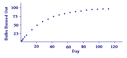
Out of curiosity (and because we own stock in the power company) we bought `100` bulbs of the same kind and started them burning at the same time. We recorded the number that had burned out after the first day, the second day, and so on through day `200`. We reproduce some of this data, mostly at one-week intervals through `16` weeks, in Table 1. By day `200`, `99` of the bulbs had burned out.

Note 1 – Light bulb failure data

9.1.1 Modeling Failure Data

We'll begin our attempt to answer lifetime questions by trying to model the function `L(t)` that represents the number of light bulbs burned out by the end of day `t`. We plot the data from Table 1 in Figure 1.

We noted in Chapter 6 that we have modeled processes that decay to a steady state in at least three settings already:

• radioactive decay,
• Newton's Law of Cooling, and
• free fall with air resistance.

In all of these previous encounters, the modeling function contained a term of the form `e^(-r t)`, where `r` is positive; the minus sign ensures that the term decays to zero as `t` increases. In the present case, it is reasonable to guess that a function of the form `M(1-e^(-rt))` should approximate `L text[(] t text[)]`.

Activity 1

Use your graphing tool to determine appropriate values for `M` and `r` so that `LA text[(] t text[)] =M(1-e^(-rt))` is a good model for `L text[(] t text[)]`.

Comment on Activity 1

In Activity 1 we concluded that `L text[(] t text[)]`, the unknown function whose value at time (in days) is the number of burned out bulbs at that time, is closely approximated by the function

Thus, for example, `LA text[(] 44 text[)]` (about `76`) approximates the number of bulbs burned out by the end of day `44`, and `LA text[(] 5 text[)]` (about `15`) approximates the number of bulbs burned out by the end of day `5`. It follows that `LA text[(] 44 text[)]-LA text[(] 5 text[)] ~~ 61` represents the number of bulbs burned out between day `5` and day `44`. If we divide this number by `100`, we obtain the fraction of the bulbs burned out between these two days: `0.61`.

We also can obtain a fractions-burned-out function by scaling `LA`. If we define `F text[(] t text[)]` as `LA text[(] t text[)] text[/] 100`, then we have

If `a` and `b` are any numbers of days, then `F text[(] b text[)]-F text[(] a text[)]` represents the fraction of bulbs burned out between time `t=a` and time `t=b`.

Checkpoint 1

Another way of looking at this is to consider what might happen if we took another bulb of the same type out of its package, screwed it into a socket, turned it on, and left it on. Our experience with the first bulbs suggests it is reasonable to assert that the probability the bulb would burn out between time `t=a` and time `t=b` is `F text[(] b text[)] -F text[(] a text[)]`.

We are now in a position to answer two of the questions raised at the beginning of the section — that will be your task in Checkpoint 2.

Checkpoint 2