9.2.3 A Geometric Look at Failure Times

Two functions played important roles in Section 9.1: The cumulative failure fraction function

and its derivative

For reasons we will explore in the next section, `F` is called an exponential distribution function and `f` is called an exponential density function. As we will see, it is no accident that the word "density" is turning up again. Recall that density played a role in our moment and center of mass calculations in Chapter 8 — calculations that were about continuous distribution of mass. In this chapter the corresponding concept will be continuous distribution of probability.

Observe that `F text[(] 0 text[)] = 0`. (That is, at the instant we turn all the bulbs on, none has burned out yet.) Thus `F text[(] t text[)]` is the solution of the initial value problem

According to the Fundamental Theorem, this means that

For the light bulb failure functions, we could check this last formula by direct calculation. However, this is a correct conclusion about the solution `F` of any initial value problem of the form

where `f` is a continuous function. We will use this more general assertion in the next section.

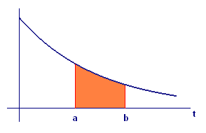
We observed in Section 9.1 that the probability of a failure between time `t=a` and time `t=b` is `F text[(] b text[)] - F text[(] a text[)]`. But that is also the value of the integral of `f` from `a` to `b`. Thus the probability of a failure between time `t=a` and time `t=b` is

where `f` is the exponential density function. This in turn gives us an interpretation of probability as area (see Figure 1): The probability of failure in a given time interval is the area under the graph of the density function over that interval.

Checkpoint 3

Example 4

Interpret expected time to failure as

1. a moment and
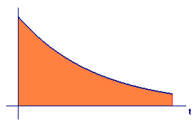
2. the center-of-mass coordinate `bar t` for the region shown in Figure 2 (extended to `oo`).

Solution   The horizontal moment for the region shown in Figure 2 is

But this is the integral expression we derived for expected failure time in the preceding section. To find `bar t` from this expression, we need to divide by the area of the region. You just showed in Checkpoint 3 that the area of the region is `1`, so in this case `bar t` and `M_y` are the same number:

One way to read this last formula is that the expected (or average) failure time is the weighted average of all possible failure times, where the weight for each `t` is given by the density function `f text[(] t text[)]`. If the sum of all the weights is `1`, one may skip the step of dividing by the sum of the weights.

Checkpoint 4