Chapter 9
Probability and Integration
9.3 Continuous Probability
9.3.1 Distribution and Density Functions
In Section 9.1 we studied data on the numbers of failures in a large collection of similar light bulbs. The key functions in our analysis of that data were
and its derivative,
The value of `F` at time `t` is approximately the fraction of bulbs that burned out by that time, so the fraction that burned out between `t = a` and `t = b` is `F text[(] b text[)] - F text[(] a text[)]`. Since `f text[(] t text[)]` is the derivative of `F text[(] t text[)]`, that fraction is also `int_a^b f text[(] t text[)] dt`. We adopted the fraction of failures in a large sample as our meaning for the probability that a randomly selected bulb would fail in a given time interval. Thus the definite integral gives us a way to describe probability for events that occur on a continuous time scale.
 The question we set out to answer in Section 9.1 was one of expected or average lifetime. We saw that average lifetime could be calculated much like a moment, as an integral giving weighted averages of times `t`, where the weights came from the function `f text[(] t text[)]`. We had to calculate these integrals over large intervals `[0,T]`, and this led to our discussion of improper integrals in Section 9.2. Now we resume our discussion of probability, and we describe the functions `f` and `F` in terms that we can use for other types of problems.
 In general terms, the distribution function `F text[(] t text[)]` describes the probability that a randomly selected data item will have a value less than `t`. (For light bulbs, "value" means "lifetime.") The probability density function `f text[(] t text[)]` is the derivative of the distribution function. Thus the probability that a random data value will fall between `t = a` and `t = b` is `F text[(] b text[)] - F text[(] a text[)]`, which is the same thing as `int_a^b
f text[(] t text[)] dt`. If `F text[(] t text[)]` is known, we find `f text[(] t text[)]` by differentiation. On the other hand, if `f text[(] t text[)]` is known, we find `F text[(] t text[)]` as a particular antiderivative of `f text[(] t text[)]`, the one that has value `0` at the left end of the domain. Thus, a probability distribution can be specified by either its distribution function or its density function.
 The expected value (also called average value) for data items from a large population with density `f` is the moment integral `int_a^b
t f text[(] t text[)] dt`, where the interval is selected to include all the possible outcomes. For example, to find the expected lifetime of light bulbs, the appropriate interval is `[0,oo)`.
 The distribution function `F text[(] t text[)] = 1 - e^(-rt)` is an exponential distribution, and its derivative `f text[(] t text[)] = re^(-rt)` is an exponential density. This model is a starting point for the study of reliability theory, which is useful for describing, among other things, failure times for electrical and electronic components such as chips in computers, batteries in toy rabbits, and bug zappers in backyards. In Example 1 in Section 9.2 we showed that the expected lifetime is exactly `1 text[/] r`. That's a measure of reliability.
Other kinds of data are distributed in other ways. In this section we study two more types of distributions and their density functions. The first of these is the Cauchy distribution (pronounced ko-SHEE), which may be defined by the Cauchy probability density function:
| for |
Activity 1
-
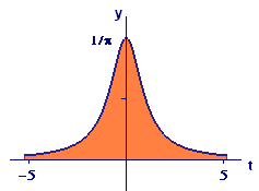
Use your graphing tool to graph the Cauchy density function `f text[(] t text[)]`.
Describe what the graph of the Cauchy density function says about the distribution of data values in a set modeled by this density function.
Show that the integral of `f` over its entire domain is `1`.
Explain why, for any probability density function `f`, the integral of `f` over its entire domain must be `1`.
Find a formula for the Cauchy distribution function `F`. [Recall that `F text[(] t text[)]` represents the probability that a random data value is less than `t`.]
Evaluate `lim_(t rarr - oo) F text[(] t text[)]` and `lim_(t rarr oo) F text[(] t text[)]`.
Explain why any distribution function `F` must be an increasing function that approaches `0` at the left end of its domain and `1` at the right end.
 |
We show the graph of the Cauchy density function in Figure 1. Now that you have a formula for the Cauchy distribution function `F text[(] t text[)]`, you can graph it as well. You should see an S shape similar to the graph of the arctangent function, but starting at `0` on the left and rising to `1` on the right.
Every distribution function must have these properties: The fraction of data values found to the left of the domain must be `0`, and the fraction found to the left of the right endpoint of the domain must be `1`. Furthermore, `F` describes a cumulative distribution, so it can never decrease. [It could stay level over some interval — if `f text[(] t text[)] = 0` there — but that doesn't happen with the Cauchy distribution.]
does not converge! (See Exercise 12 in the preceding section.)
We turn now to an example of a probability distribution that is much simpler than either the exponential or the Cauchy distribution. In fact, this example is so simple it is child's play. Figure 2 shows the spinner (slightly modified) from the popular children's game Chutes and Ladders®. Its purpose is the select a random integer from 1 to 6. However, note that each of the six wedges is already subdivided into fifths, and we can easily imagine that each wedge could be divided into tenths or even finer. If we associate the "1" wedge with the interval `[0,1]`, "2" with `[1,2]`, and so on, we can view the spinner as randomly selecting a number between `0` and `6`. (As shown, the arrow is pointing slightly below `0.9`.) You can easily decide whether the result of a spin is, say, greater than `2.3` and less than `3.6`.

Figure 2 Chutes and Ladders spinner
We assume that this is a "fair" spinner for example, the result of a spin is as likely to give a value greater than `3` as a value less than `3`. More generally, given two intervals of equal length, the probability of landing in one is the same as that for landing in the other. We suppose that we have a data set that consists of the numerical results from a large number of spins.
Activity 2
Explain why, for the spinner data just described, a reasonable density function is
`f text[(] t text[)] = 1/6` for `0 ≤ t ≤ 6`.
What is the distribution function?
Find the expected value for a random result from the spinner. Does your result agree with the value you would have assigned intuitively?
The type of distribution represented by the spinner data is called a uniform distribution, and the corresponding density function is called a uniform density function. A uniform density function must be constant on some interval of finite length, with the product of the length and the constant height equal to `1`. The distribution function is linear with slope determined by the constant height of the density.


