Section 9-3 Exercises

Chapter 9
Probability and Integration

9.3 Continuous Probability

Exercises

If `Ftext[(]t text[)]=1-e^(-rt)` is the failure distribution function for light bulbs with an expected lifetime of 800 hours and time is measured in days, what is `r`?

In the text we gave no application or physical interpretation of the Cauchy distribution. We ask you to explore that now with the game spinner we modeled by the uniform distribution (see Figure E1). However, instead of reading numbers from the spinner, we read slopes. Specifically, wherever the arrow ends up, look only at the right-hand half of it — whether that is the arrow end or not. Think of it as a line in the right half of the plane. For any run `Delta x` there is a corresponding rise `Delta y` (which might be negative). Calculate the slope `Delta y`/`Delta x`. That's the "value" of a spin.

Figure E1 A game spinner
1. Explain why data values can range from `-oo` to `oo`. Where would you expect to find most of the data values clustered? What symmetry do you observe?
2. Show that the slope data values are distributed according to the Cauchy distribution. That is, show that the probability of a slope between `a` and `b` is
  `1/pi (tan^(-1) b-tan^(-1) a)`.

Let `f` be a probability density function given by `ftext[(]xtext[)]=cx` for `1<=x<=5`.
1. Find `c`.
2. Find a formula for the distribution function.
3. What is the probability of the event occurring between 2 and 3.5?
4. Find the expected value.

If `ftext[(]t text[)]=c(6t-t^2)` is a probability density function over the interval `0<=t<=6`, find `c`.

Figure E2 shows two graphs, one of which is a probability density function and the other of which is a probability distribution function. Which is which? Identify as many features as you can of each graph that help you make the proper identification.

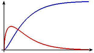
Figure E2 Probability density and distribution functions

In this exercise we introduce the following notation: `P(A)` stands for the probability that the event `A` happens. `P(A and B)` stands for the probability that both events `A` and `B` happen. `P(A|B)`, which we read "probability of `A` given `B`," stands for the probability that event `A` happens given that `B` has already happened.
1. Show that if `P(B) = ``1/3` and `P(A and B)=``1/6`, then `P(A|B)=``1/2`.
2. Explain why, if and are random events, then in general
  `P(A|B)=(P(A and B))/(P(B))`.

Suppose a product has a life span that is distributed exponentially with `t` measured in years, i.e., `ftext[(]t text[)]=r e^(-rt)`.
1. Find the probability that the product will fail in the first year.
2. Suppose the product has already lasted five years — i.e., it did not fail during the first five years. What is the probability that it will fail within the next year? (See the preceding exercise.)
3. Show that the probability of failing in the first `k` years is the same as the probability of failing in `k` additional years, given it has already lasted `n` years.
4. Discuss the implications of the result in part (c).

Suppose `f` is a probability density function that models the following situation: `x` can take on any value between `1` and `10` and only those values. The probability of a value occurring in any two intervals of the same length is the same. Write down a formula for `f`.

Suppose that your company expects to sell about 300,000 computer chips over the next year. Your statisticians have determined that the following function represents the fraction of the total number of computer chips that will have failed as of time `t` (in months): `Ftext[(]t text[)]=1-e^(-0.008 t)`.
1. How many chips would you expect to last more than a year?
2. On average, how long would you expect a computer chip to last?
3. Does it make sense for your company to offer a one-year guarantee on these chips? Explain.

Observations of traffic on limited access highways have shown that the time gaps between successive cars tend to be exponentially distributed. Suppose the observed average time gap on a certain highway is 10 seconds.
1. What is the probability density function for time gaps?
2. What is the distribution function?
3. What is the median time gap?
4. What is the probability that a gap between cars will exceed 30 seconds?
5. What is the probability that a gap between cars will be seconds or less?

There is an old saying that "A watched pot never boils." In a recent (fictional) study it was discovered that the probability that a watched pot boiled in the first minute is `1//2`. That is, if `T` represents the number of minutes until the pot boils, then `P(0<=T<1)=1text[/]2.` Furthermore, scientists established that the probability density function is of the form

`ftext[(]t text[)]=c/(1+t^2)`.
1. Find `c` by using the fact that `P(0<=T<1)=1text[/]2.`
2. Find the distribution function.
3. According to this research, what is the expected time for a pot to boil? What does your answer imply about the old saying?

Problem contributed by Sam Morris, Duke University.

Suppose you have a normally distributed data set with mean `10` and standard deviation `2`. What is the probability that a random data value will be
1. between `9` and `12`?
2. less than `9.7`?
3. greater than `9.7`?
4. between `9.3` and `11.5`?

Find the mean and the standard deviation for each of the following data sets.

Table E1 Scores on a mathematics
examination with 200 points maximum
200	200	200	190	186	170
167	165	164	159	159	147
146	144	131	128	124	109

Table E2 Maximum daily temperatures
during a week in July
94	93	95	85	87	90	95

Table E3 Annual rainfall in England
Year	1992	1993	1994	1995	1996	1997	1998	1999	2000	2001	2002
Rainfall (millimeters)	872	914	930	765	683	790	963	914	1,078	848	988

Table E4 Annual rainfall in Scotland
Year	1992	1993	1994	1995	1996	1997	1998	1999	2000	2001	2002
Rainfall (millimeters)	1,738	1,493	1,608	1,493	1,264	1,422	1,738	1,666	1,594	1,264	1,551

Source for Tables E3 and E4: UK National Statistics, retrieved 4/4/07

What is the probability that a random data value from a normally distributed data set will lie within one standard deviation of the mean? That is, what is the probability that `|value-m|<sd`?

What is the probability that a random data value from a normally distributed data set will lie within 1.5 standard deviations of the mean? within 2 standard deviations of the mean? within 3 standard deviations of the mean?

Explain the following rules of thumb for normal distributions: About 68% of the data values are within one standard deviation of the mean, about 95% within two standard deviations, and about 99% within three standard deviations.

Suppose a data set has the standard normal distribution. Find a number `w` such that the probability that a random data value is greater than `w` is `1//3`.

Suppose a data set has the standard normal distribution. Find a number `w` such that the probability that a random data value is less than `w` is `1//10`.

Suppose a data set has a normal distribution mean `3` and standard deviation `0.5`. Find a number `w` such that the probability that a random data value is less than `w` is `1//10`.

Suppose a data set has a normal distribution mean `3` and standard deviation `0.5`. Find a number `w` such that the probability that a random data value is greater than `w` is `1//5`.

IQ scores are supposed to be normally distributed with mean 100 and standard deviation 15. What percentage of the population has an IQ
1. between 100 and 110?
2. less than 90?
3. between 115 and 125?
4. more than 140?

Write the standard normal distribution function,
`Ftext[(]t text[)]=1/2+int_0^t ce^(-s^2text[/]2) ds`,
in terms of the error function.

Find the points of inflection of the graph of the standard normal density function.

Table E5 Heights of 1253 boys
Height (inches)	Number
46	1
47	3
48	7
49	13
50	31
51	73
52	111
53	176
54	189
55	198
56	162
57	106
58	77
59	49
60	31
61	10
62	9
63	4
64	1
65	1
66	1

Toward the end of the 19th century, H. P. Bowditch measured the heights of 1253 eleven-year-old boys. We show these data in Table E5 and a histogram plot in Figure E3.

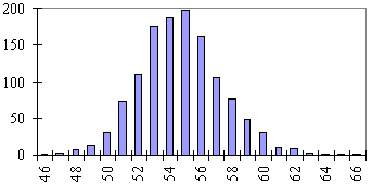
Figure E3 Histogram of Bowditch data

Find the mean and standard deviation of this data set.
If the data are normally distributed, how many boys would you expect to have heights of 57 inches or more? How many boys had heights of 57 inches or more?
Do you think these data are normally distributed? Carry out two more experiments similar to the one in (b) to see if your opinion is supported.

Adapted from Statistical Reasoning by Gary Smith, Allyn and Bacon, Inc., 1985. The data appeared in H. P. Bowditch, "The Growth of Children," Report of the Board of Health of Massachusetts, VIII, 1877.

Which of the data sets in Tables E1 – E4 do you think might be normally distributed? Explain your conclusions.

In 1983, Camilla Benbow and Julian Stanley published in Science a study of almost 40,000 seventh-grade students who had taken the mathematics section of the Scholastic Aptitude Test (SAT-M) in the three preceding years. Their results, separated by gender, are shown in Figure E4: Each group had normally distributed scores with a standard deviation of 60. The boys had a mean of 412 and the girls a mean of 385. A standard statistical test shows that these means are significantly different. Benbow and Stanley's controversial conclusion was that this showed "endogenous" male superiority in mathematical ability. For purposes of this exercise, we concede the point that there is a gender difference here, and we ignore questions of
- what the test measures,
- whether the boys and girls had the same educational experiences or levels of encouragement, and
- whether the sample of students was unbiased.
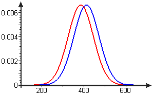
The question we address is the predictiveness of the measurement.

Figure E4 Boys' and girls' SAT-M scores
1. Suppose you had no knowledge of the Benbow-Stanley study, and, for random boy-girl pairs of seventh-graders, you guess which will have the higher SAT-M score. How often would you expect to be right?
2. Suppose instead, for your random boy-girl pairs, you always assume that the boy will have the higher score. How often would you expect to be right? Describe in your own words the gain in predictiveness that results from knowing the Benbow-Stanley result.
3. How would you compare the difference between genders with the variability within genders? Think of appropriate numerical measures, and describe your comparison in words.
Note 2 – Sources and further comments

Explain why any probability density function of the form `ftext[(]t text[)]=ce^(-t^2text[/]b)` must have zero as its expected value (mean). You should be able to explain this without calculating an integral, but calculate an integral if you must.

Suppose `m` is the mean and `sd` is the standard deviation for a normal distribution. Define `f` by
`ftext[(]t text[)]=c/(sd) text[exp][(-text[(]t-mtext[)]^2)/(2 sd^2)]`,
where `c` is the constant that appears in the definition of the standard normal density function.
1. Show that for any `a<b`, `int_a^b ftext[(]t text[)] dt=int_c^d gtext[(]u text[)] du`, where `g` is the probability density function for the standard normal distribution, `c=(a-m)/(sd)`, and `d=(b-m)/(sd)`.
2. Explain why the calculation in (a) verifies that `f` is the probability density function for the normal distribution with mean `m` and standard deviation `sd`.

Recall that the mean or expected value of a continuous probability distribution with density function `ftext[(]t text[)]` defined from `-oo` to `oo` is `mu=int_(-oo)^(oo) t ftext[(]t text[)] dt`, a weighted average of the values of `t`, with `ftext[(]t text[)]` serving as the weight function. [This mean is denoted by the Greek lower-case mu, `mu`, to distinguish it from the mean `m` of a sample of data from the population with density `ftext[(]t text[)]`.] The variance of the distribution is the weighted average (in the same sense) of squared distances from the mean — that is, the variance is
`int_(-oo)^(oo) text[(]t-mutext[)]^2 ftext[(]t text[)] dt`.
Not surprisingly, the square root of the variance is called the standard deviation of the distribution. Show that the standard deviation of the standard normal distribution with probability density function `ftext[(]t text[)]=0.3989 e^(-t^2text[/]2)` is `1`.

Consider the following process: We select an individual at random from among the population of healthy adults, and we have that individual run or jog for as long as he or she can and then stop. We don't know the distribution for this process, but we can imagine that the probability density function has the form shown in Figure E5, namely, a function of the form `ftext[(]t text[)]=k e^(-t^2text[/]2)`, where `k` is a constant, and `t` represents time in hours.

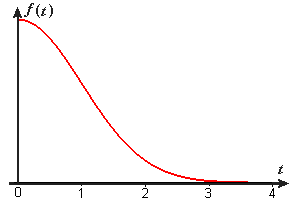
Figure E5 `ftext[(]t text[)]=k e^(-t^2text[/]2)` for `0<=t<oo`
1. What is the value of `k`? (Think about how this density function is related to the normal probability density function.)
2. Make a rough sketch of the distribution function whose density function is `ftext[(]t text[)]`.
3. Find the mean (or expected) time that a random individual can run.
4. Determine the probability that a randomly selected individual can run no longer than the mean time for the whole population.

Image credits

Contents for Chapter 9

Chapter 9 Probability and Integration

9.3 Continuous Probability

Chapter 9
Probability and Integration