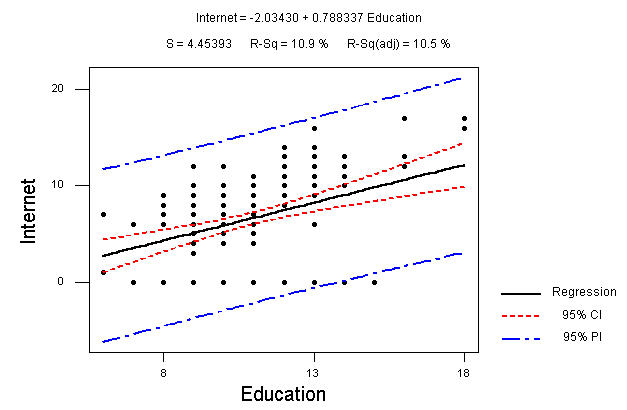
Results for: xr18-08.txt

Regression Analysis: Internet versus Education


The regression equation is
Internet = - 2.03 + 0.788 Education

Predictor        Coef     SE Coef          T        P
Constant       -2.034       1.791      -1.14    0.257
Educatio       0.7883      0.1598       4.93    0.000

S = 4.454       R-Sq = 10.9%     R-Sq(adj) = 10.5%
Here's the picture:
Since the constant term was not significant at an alpha of .05, we might rerun the model without the constant term (under Options, uncheck "Fit Intercept"):
Regression Analysis: Internet versus Education


The regression equation is
Internet = 0.610 Education

Predictor        Coef     SE Coef          T        P
Noconstant
Educatio      0.60969     0.02812      21.68    0.000
Because all those zeros mean we have people not participating in the internet, we might decide to change our focus and talk about only those who USE the internet. After removing those people, we obtain a much better model:
Regression Analysis: i_culled versus e_culled


The regression equation is
i_culled = - 1.39 + 0.950 e_culled

Predictor        Coef     SE Coef          T        P
Constant      -1.3878      0.9427      -1.47    0.143
e_culled      0.94967     0.08375      11.34    0.000

S = 2.031       R-Sq = 47.2%     R-Sq(adj) = 46.8%
Here's the picture:
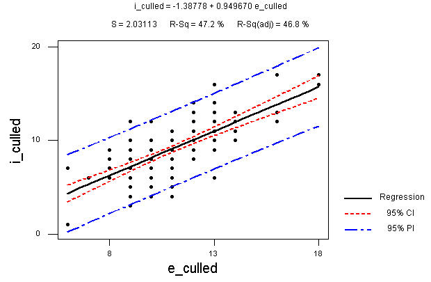
Note that the prediction intervals now are much tighter. This is a much improved model!
Again, the constant is not significant, so we might drop it and rerun the analysis:
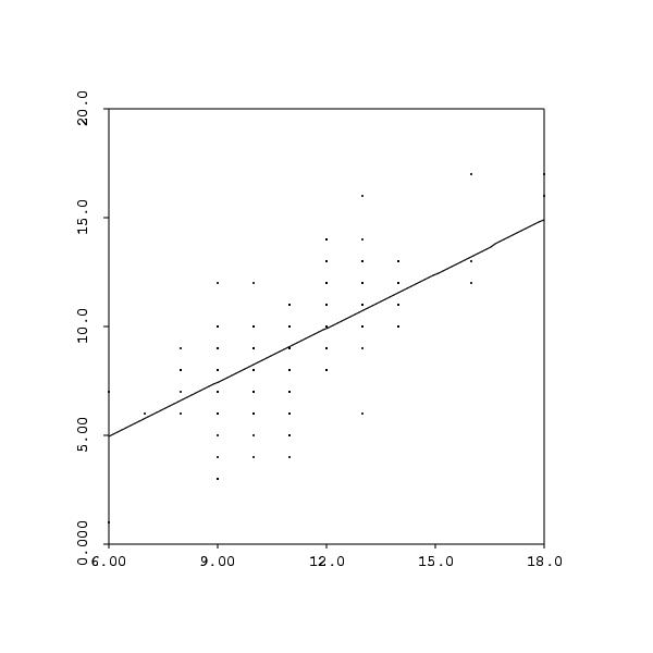
Regression Analysis: i_culled versus e_culled


The regression equation is
i_culled = 0.828 e_culled

Predictor        Coef     SE Coef          T        P
Noconstant
e_culled      0.82835     0.01499      55.24    0.000
(unfortunately it seems that Minitab doesn't ordinarily produce a fitted-line plot in the case of no constant, although it would be easy for them to do):
We can now use the model to predict at various points: here's the prediction of internet use for high school graduates (education = 12) and college grads (education = 16):
Predicted Values for New Observations

New Obs     Fit     SE Fit         95.0% CI             95.0% PI
1         9.940      0.180   (   9.585,  10.296)  (   5.894,  13.986)
2        13.254      0.240   (  12.779,  13.728)  (   9.195,  17.312)

Values of Predictors for New Observations

New Obs  e_culled
1            12.0
2            16.0
The CI is for the average of those years of education; the PI (Prediction Interval) is for a single point. Hence for high school students the mean, based on our data, is between ( 9.585, 10.296) hours with 95% confidence. If your brother just graduated from high school, we might predict with 95% confidence that his use will fall within ( 5.894, 13.986) hours.