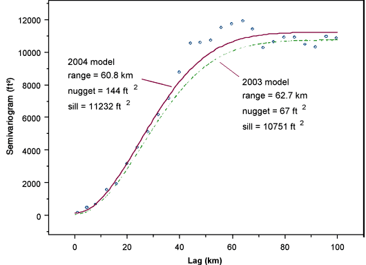
The Variogram: a spatial decomposition of variance
Suppose that we have measured the variables $z$ at $N$ locations, whose
geographical positions are denoted $\underline{x}_i$. Consider all pairs of
data locations, of which there are $N_p=\frac{N(N-1)}{2}$.
Now each pair of data locations is placed into a "lag class",
determined by a vector $\underline{h}$ (the "lag"), which means that
the two points are separated by (roughly) $\underline{h}$. Define
$N_c$ classes, each described by a set $P_{\underline{h}}$ of pairs of
indices, such that
$
(i,j) \in P_{\underline{h}}
\iff
\underline{x}_i-\underline{x}_j \approx \underline{h}.
$
The univariate variogram is defined as
$
\gamma(\underline{h}) = {\frac{1}{2}}E \left [(z
(\underline{x}+\underline{h})-z(\underline{x}))^2 \right ]
$
and the estimator of the variogram function for lag $\underline{h}$ is
$
\gamma(\underline{h})={\frac{1}{2N_{\underline{h}}}}\, \, \, \sum_{(i,j)\in P_{\underline{h}}}^{N_{\underline{h}}}(z_i-z_j)^2,
$
where $N_{\underline{h}}$ is the number of distinct pairs of data values,
placed in the set $P_{\underline{h}}$ (pairs displaced by the vector
$\underline{h}$). $\gamma(\underline{h})$ is sometimes called the
semi-variogram, because of the factor of 1/2 in its definition.
Now the sample variance, $s^2$, can be written as a weighted sum
$
s^2 = \sum_{c=1}^{N_c} \left({\frac{N_{\underline{h}}}{N_p}}\right) \left( {\frac{1}{2N_{\underline{h}}}}\, \, \,
\sum_{(i,j)\in P_{\underline{h}}}^{N_{\underline{h}}}
(z_{i}-z_j)^2 \right),
$
or
$
s^2 = \sum_{c=1}^{N_c} \gamma(\underline{h}) \left (\frac{N_{\underline{h}}}{N_p}}\right).
$
It is this equation which leads me to declare that
The sample variogram is the spatial decomposition of the sample variance.


