More about Ipop

Moran’s I adjusted for population size

A test for spatial autocorrelation in disease rates that accounts for geographic variation in population size.

Data Requirements

Population sizes and disease rates

Link file with connection weights, rules are as follows:

when 2 cases are in the same area the weight assigned is w_ii=2/d_i

weights for 2 different areas, i and j, are set to w_ij unless otherwise specified
weights read from the connection file are divided by

Number of Monte Carlo runs

Analysis

H₀: probability of a case occurring in an area is given by the proportion of the total population in that area, or in other words, the geographic variation in the number of cases is expected to follow geographic variation in population size

H_a: geographic variation in the number of cases does not follow geographic variation in population size

Test Statistic: I_pop is a spatial autocorrelation coefficient adjusted for the size of the population at risk.

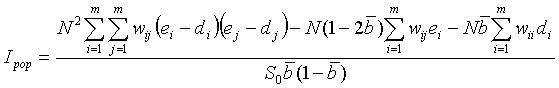
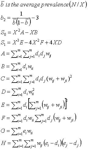
where m is the number of regions, N is the total number of cases in all of the regions, n_i is the number of cases in area i, i is the proportion of cases in area i (e_i = n_i/N), X is the total size of the risk population in all of the areas, x_i is the size of the risk population in area i, d_i is the proportion of the population in area i (d_i = x_i/X), e_i – d_i is the difference between the proportion of cases in area i and the number of cases expected given the areas population size, w_ij is the weight for areas i and j (the weights describe the alternative spatial model defining how ‘connected’ the areas are), and:

Large values of I_pop indicate positive spatial autocorrelation or similar rates in connected areas; small values indicate negative spatial autocorrelation or dissimilar rates in connected areas. I_pop is large under two clustering scenarios, first, when cases cluster within counties (because e_i – d_i becomes large) and second, when regions with may cases are adjacent. The range of I_pop depends on population size, and it is useful the standardize the statistic using:

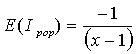
Expectation of I_pop under H₀ is:

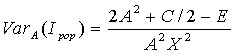
The variance of I_pop under H₀ is:

An approximation can also be calculated for the variance:

Significance is evaluated using three approaches: by Monte Carlo simulation, under the randomization assumption and by approximation. Under simulation the cases are allocated at random among the regions according to the proportion of the total population in each region. Under the randomization assumption a z-score can be calculated as the difference between the observed and expected value of I_pop in standard deviation units. A two-tailed p-value is reported because spatial pattern is of interest both when I_pop is positive or negative.

Output

I_pop, I_pop’, E[I_pop]

Variance and significance under randomization assumption, approximation, and simulation

Plot of frequency distribution of I_pop obtained under simulation

Reference

Jacquez, G.M. 1994, User manual for Stat!: Statistical software for the clustering of health events, BioMedware, Ann Arbor, MI.