Ø N : Number of cases
Ø
![]()
Ø
![]()
Ø
![]()
Ø
![]()
Ø
X : The test statistic,
 .
.
Knox method
Description: The Knox method quantifies space-time interaction based on critical space and time distances. The test statistic, X, is a count of those pairs of cases that are separated by less than the critical space and time distances. Pairs of cases will be near to one another when interaction is present, and the test statistic will be large.
Notation:
Ø N : Number of cases
Ø
![]()
Ø
![]()
Ø
![]()
Ø
![]()
Ø
X : The test statistic,
 .
.
Null hypothesis: The times of occurrence of the health events are distributed randomly across the case locations. This is another way of saying the time distances between pairs of cases are independent of the spatial distances between pairs of cases. The null distribution of X is constructed under an approximate randomization which permutes the row-column elements of the time adjacency matrix while holding the space adjacencies constant. This procedure is accomplished `Number of runs' times, and X is calculated each time from the newly randomized data.
Significance: The probability value is the proportion of the upper right hand tail of the null distribution whose X values are as large or larger than the test statistic. Let NGE be the number of X values under simulation that were larger than X obtained from the original (not randomized) data. Nruns is the number of simulations. The P-value is

Data screen: Let's apply Knox's test to the disease data in `Epidemic.pnt'. This example assumes you have already calculated the geographic and time distance matrices `Epidemic.geo' and `Epidemic.tmp' using the distance method. If you haven't, turn to the section titled `Distance method' in this Chapter and calculate the distance matrices. Access the Knox data screen by selecting `Space-time' from the horizontal method menu, then `Knox' and `Data'.
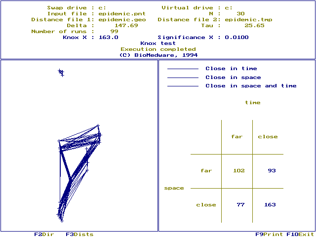
Enter the names of two distance files and the point (pnt) file (optional) from which they were calculated. Case locations in the point file will be used to create a linkage map. If you don't enter a point file name the linkage map won't be shown. `Number of runs' is the number of replicates used to determine the null distribution of the test statistic, set it to 99. `Display links' determines the kinds of connection between pairs of cases that will be displayed after the calculations complete. Displaying links near in space and time will connect those pairs of cases that contribute to Knox's X.
Selecting a critical distance: You also need to enter critical space and time distances in the `Critical distance' fields. Distance file 1 is a geographic distance matrix (`Epidemic.geo'), and the critical distance you enter in the row titled `Distance file 1' must be a critical geographic distance (![]() ). Distance file 2 is a time distance matrix (`Epidemic.tmp') and the critical distance you enter in the row `Distance file 2' must be a critical time distance (
). Distance file 2 is a time distance matrix (`Epidemic.tmp') and the critical distance you enter in the row `Distance file 2' must be a critical time distance (![]() ).
).
Knox designed this method to account for latency periods. A latency period is the time between exposure and the manifestation of symptoms. If you suspect a disease with a latency period of 3 days set the time critical distance long enough to allow symptoms to appear, say 4 or 5 days. For infectious diseases, the geographic critical distance reflects the average distance between 2 individuals, one of whom infected the other. In general, one selects critical distances consistent with the disease hypothesis under investigation. This hypothesis based approach avoids problems of subjectivity which arise when critical values are determined from the data.
However, when knowledge of the underlying disease process is absent critical values can be quantified based on the distributions of space and time distances. This approach is crude and should only be used when an epidemiologic hypothesis is lacking. In these instances use the mean geographic distance for ![]() and the mean time distance for
and the mean time distance for ![]() . You can systematically vary the critical distances to identify those values that maximize Knox's X. This can provide insight into the spatial and temporal scale of the disease process, but precludes any formal evaluation of statistical significance because of multiple tests. Do not choose critical distances larger than the maximum distance in the data, since the number of cases near in both space and time will always be zero. Stat! will not accept critical distances that are outside the minimum and maximum distances observed in the data.
. You can systematically vary the critical distances to identify those values that maximize Knox's X. This can provide insight into the spatial and temporal scale of the disease process, but precludes any formal evaluation of statistical significance because of multiple tests. Do not choose critical distances larger than the maximum distance in the data, since the number of cases near in both space and time will always be zero. Stat! will not accept critical distances that are outside the minimum and maximum distances observed in the data.
We have no epidemiologic knowledge to support a choice of critical distance, and instead use the mean values as shown on the data screen. Press `F10' to exit the data entry screen, and select `Run'. The calculations will take a moment as the simulations are conducted.

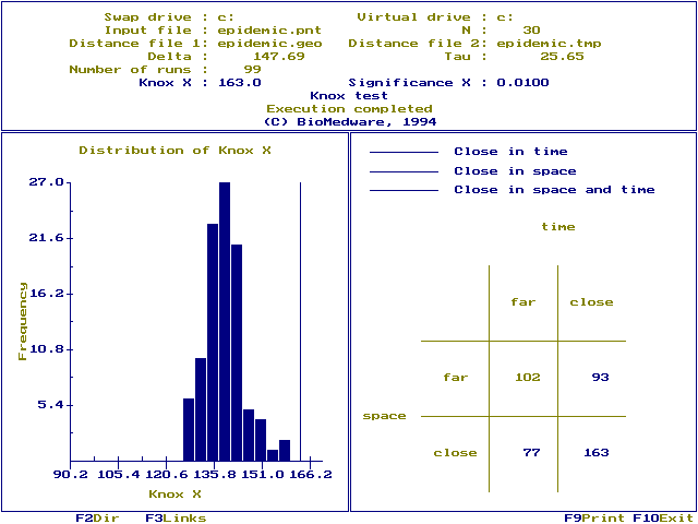
Run screen: The significance of X is shown in the top window. Significance values may vary somewhat under the approximate randomization. You can reduce this variation by selecting larger `Number of runs'. Notice the maximum P-value that can be resolved depends on the numbers of runs. We choose Nruns=99, which means the maximum P-value we can resolve is P=0.01, calculated as ![]() . You would need 999 runs to resolve P-values as small as 0.001. The P-value is a one-tailed probability corresponding to space-time interaction. Also displayed are the swap and virtual drives, the input file (`Epidemic.pnt'), number of cases (30), distance files (`epidemic.geo', `epidemic.tmp'), critical distances (147.69, 25.65) and the number of runs used in the randomization (99)
. You would need 999 runs to resolve P-values as small as 0.001. The P-value is a one-tailed probability corresponding to space-time interaction. Also displayed are the swap and virtual drives, the input file (`Epidemic.pnt'), number of cases (30), distance files (`epidemic.geo', `epidemic.tmp'), critical distances (147.69, 25.65) and the number of runs used in the randomization (99)
A 2 x 2 contingency table is shown in the right window. 93 case pairs are far in space and close in time, 77 are close in space and far in time, and 163 pairs are close both in space and time (Knox X=163). Entries in the contingency table are color coded to identify which pairs are near or far in space and time, using the following system:
| Space | Time | Color variable |
| Close | Far | Links |
| Far | Close | Point |
| Close | Close | Cases |
| Far | Far | Controls |

The colors for `links', `point' and so on are assigned on the color data entry screen, accessed via `System' on the horizontal methods menu (see the `Colors' section in Chapter 3).
Function key [F3] displays a linkage map. Which links are displayed is determined by `Display links' on the data screen. We choose to display those links that were near in space and time. This means only those pairs of cases contributing to Knox's X are linked.
The histogram (window on left of screen) shows the frequency distribution of X under the null hypothesis of no association between the space and time adjacencies. The test statistic is shown as a vertical line on the distribution. When space-time interaction is present this line will be to the right of the distribution. The P-value (0.01) is small and significant, and Knox's X is well to the right of its null distribution. We conclude space-time interaction exists in these data.
References:
Knox, G. 1963. Detection of low intensity epidemicity: application to cleft lip and palate. British Journal of Preventive and Social Medicine, 18:17-24.