Direction Method Example Analysis
Direction method
�
Description:
The direction method is used to
determine the average direction of advance of a spread of cases. A chain of
infection is constructed by first sequencing the cases by time of
occurrence. The earliest case would be first, followed by the second case
and so on. An arrow is then drawn from the location of the first case to
the location of the second case, and this is repeated until all cases are
connected. The chain of infection has at least two ends (the first and
last cases), and branches when cases occur at exactly the same time. The
test statistic is a vector whose direction is the average direction of the
arrows comprising the chain of infection, and whose magnitude is the angular
variance of these arrows. When the arrows all point in the same direction
the angular variance is small, and when they point in many directions the
angular variance is large. The method is sensitive to a systematic,
directional spread of cases. This pattern occurs when an epidemic sweeps
through an area. It also arises from geographically localized exposures,
with individuals near the source receiving higher doses and showing symptoms
before those further from the source. In this section the term `chain of
infection' is used loosely to describe the sequence of occurrence of cases.
It does not imply that the sequence of cases was the result of an infectious
disease.
�
Notation:
Ø
(xi, yi): Geographic coordinates of case i.
Ø
Dxij
: Distance on x axis between cases i and j,
Dxij = xi-xj
Ø
Dyij
: Distance on y axis between cases i and j,
Dyij = yi-yj
Ø
Qij
: Angle between a horizontal line and the vector connecting cases i and j
Ø

Ø

Ø
C: Cosine matrix whose elements are cij.
Ø
S: Sine matrix whose elements are sij
Ø
T: Time connection matrix describing the proximity, in time, of the cases to one another (see below).
Ø
v: The test statistic is a vector pointing in the average direction of advance of the chain of infection:

The vector v points in the average direction of advance of the spread of cases, and its magnitude (termed the angular concentration) represents the variance in the angles between connected cases. When the magnitude is small the variance in the angles is large, and when the magnitude is large the variance in the angles is small. Angles are taken as counter clockwise degrees from horizontal, with East corresponding to 0 and North to 90. Concentration is in the range of 0 to 1, with 1 indicating an angular variance of 0. A consistent direction of spread of cases will result in an angular concentration near 1. A random spread of cases will result in an angular concentration near 0.
�
Time connection matrix: Suppose N cases occur at times (t1,...tN). The elements of the time connection matrix are determined by the researcher to reflect the suspected temporal scale of the pattern. The alternative directed time measures are:
| ØRelative |
tij= |
| 1 if tj > ti |
| 0 if tj = ti |
| -1 if tj < ti |
|
| ØAdjacent |
tij= |
| 1 if tj is just after ti |
| 0 otherwise.
|
| -1 if tj is just before ti |
|
| ØFollowing |
tij= |
| 1 if tj is just after ti |
| 0 otherwise.
|
|
Use relative when you wish to include the vectors connecting each case to all of the cases that follow it. This is appropriate when you hypothesize a directional process operating on a longer time span. You are connecting cases that may be several links removed in the chain of infection.
Use adjacent when you wish to connect each case only to it's temporal nearest neighbors. These are the cases that occur just before and just after the case. This is appropriate when you hypothesize directional effects of short duration.
Use following when you wish to connect each case only to the case (or cases) that immediately follow it. This is appropriate when you wish to trace the average direction of the chain of infection.
�
Null hypothesis: The directions of the vectors connecting pairs of
cases are independent of the times at which the cases occur. In other
words, the null spatial model states that the direction of the axis drawn
between two cases is independent of when the two cases occurred.
�
Significance: The significance of the average
direction is evaluated through a randomization procedure which holds the
sine and cosine matrices constant and randomly assigns connections between
pairs of cases. This is equivalent to holding the locations of the cases
fixed while randomizing their times of occurrence. This randomization
procedure is repeated to generate a distribution of the angular
concentration under the null hypothesis. A P-value is determined by
comparing the angular concentration from the original (not randomized) data
to this null distribution. Let NGE by the number of times the
angular concentration under simulation was greater than or equal to
the angular concentration obtained from the original data. Nruns
is the number of simulations. The P-value is then

�
Input screen: Select `Space-time' from the horizontal methods menu,
then `Direction' and `Data' to display the direction data entry screen.
You need to enter the name of the point file containing the locations and
times of occurrence of the cases (`Wave.pnt') and the number of runs to use
when generating the null distribution (249). You also must choose the
directed time measure that will be used to generate the time connection
matrix. The alternatives are relative, adjacent and following. The data
in `Wave.pnt' describe an infectious disease that originated in the
south-west corner of a study area. You believe the cases spread northward
from this initial focus, and you would like to determine the direction of
the spread of cases. Choose `adjacent' for the directed time measure.
This will include vectors connecting each case to the cases that immediately
preceded or followed it.
�
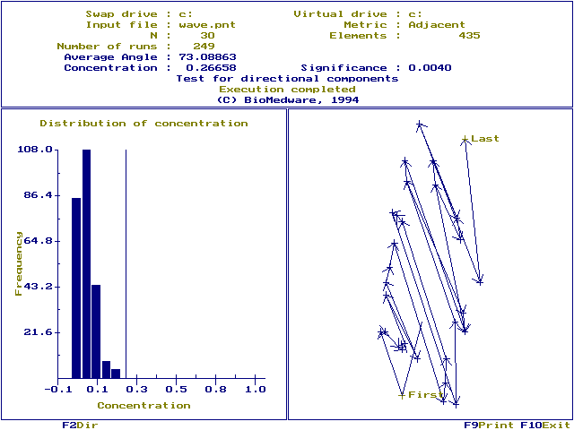
Run screen: Press `F10' to exit the data entry
screen, and select `Run'. The 249 simulations will begin, and the null
distribution of the angular concentration will be constructed in the window
on the left of the run screen. Examine the top window while the
simulations run. It shows the input file (`wave.pnt'), the directed time
measure (`Adjacent'), the number of cases (30) and the number of elements in
the sine and cosine matrices (435). It also displays the number of runs
used to evaluate significance (249), the average angle (73.08863), the
angular concentration (0.26658) and the significance (0.0040).

The chain of infection is shown in the lower right hand window. The first case occurs in the south of the map and the last case occurs in the north. There appears to be a systematic progression of cases in a Northerly direction. The average angle is shown on the map as a vector with the first case at its tail, and pointing in the average direction of advance. But is this pattern statistically significant?
To answer this question we examine the frequency distribution shown in the left window. This is the distribution of concentration expected under the null hypothesis of no association between the angles from case to case and the times at which the cases occurred. An average angle will always be calculated whether or not there is a systematic direction to the spread of cases, and is meaningful only when the concentration is statistically significant. The observed concentration (0.26658 for these data) is shown as a vertical line to the right of the distribution, and is significant (P=0.0040). We conclude the cases spread along an average angle of 73.00863.
�
Notes: A significant angular
concentration can arise whenever case location depends on the locations of
preceding cases, and does not necessarily mean there was an underlying
directional process. For example, a simple random walk may result in
statistical significance whenever the walk starts in one place and ends up
somewhere else. Although the walk is undirected, the spread of cases has a
significant, average direction. You cannot infer a directional process
from the direction test, you can, however, determine whether the observed
spread of cases tends to be in one direction.
Website maintained by Andy Long.
Comments appreciated.


