


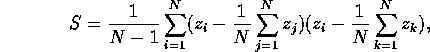
We derive this decomposition as follows, starting with the sample variance S computed by the usual formula:
![]()
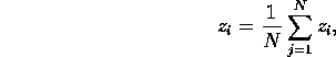
Replacing the mean ![]() by the sum which defines it,
by the sum which defines it,
Since
and so
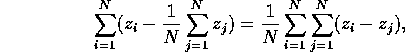
we can rewrite S as
Adding an appropriate form of zero (my favorite trick),
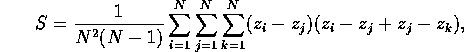
which is

Notice that the second sum as exactly S, so
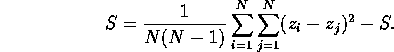
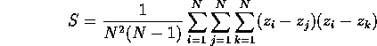
We solve for S,
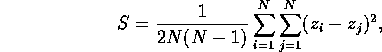
and replace the redundent pair information by a factor of two (note the change on the index of j) to yield
where ![]() is the total number of distinct pairs of data positions, of which
there are
is the total number of distinct pairs of data positions, of which
there are ![]() .
.
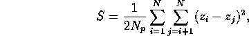
This says that the sample variance is half the mean interpair difference squared. If we now break our pairs into C classes by the vectors which separate them, then we obtain estimates of values of the variogram function.
The estimator of the variogram function for lag ![]() (that is, for
those pairs separted by a vector
(that is, for
those pairs separted by a vector ![]() ) is
) is
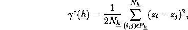
where ![]() is the number of distinct pairs of data values, placed in the
set
is the number of distinct pairs of data values, placed in the
set ![]() (pairs displaced by the vector
(pairs displaced by the vector ![]() )
)
Thus the sample variance, S, can be written as a weighted sum
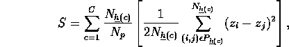
or
![]()