Day 03 in Mat360

Today:

• Announcements:
  • Your first homework set is due.

    As a rule, please fold your homework in half the long way, and set t on the table in front at the beginning of class.

  • You have an assignment due next Tuesday, as well. Questions?

  • I've gotten many of your appendix files (but not all).
    • Michael W. had an interesting comment/question: "The way I did it, the answers came after all the commands per section. Not sure how to get the answer to come after each command."

      Let's take a look at his file, and see!

    • What other issues arose? Are there files that "barfed" (that's a technical term!:).

• Last time we talked about algorithms, and saw an example of one that
  • Solved a problem, and
  • suggested some general principles (e.g. fixed point iteration, recursion, using graphs to illustrate a method, simple Mathematica code for solving recursive problems, etc.).
  The example also showed that errors may be, in a sense, "self-correcting". We'll discover that there are algorithms for which errors may grow, until the "solution" has no apparent relationship with the solution.

  You already know that in math there are "solutions" that are not, in fact, useful solutions! As an example, we frequently encounter "solutions" outside the domain of the independent variable in calculus.

• Section 1.4: Error

  Last time we got started talking about errors. First we conceptualize them, then we quantify them, and of course we look at some examples.

  We're going to make them, so we have to keep them front and center. It's an odd place to spend so much time, isn't it? I'm sure that some of you are thinking that this is not the pristine math you've grown up with...:)

  Important questions:

  • How do we define errors?
  • How do we measure errors?
  • How do we avoid errors?
  • How do we prepare for errors?
  • How do we minimize errors (since we're guaranteed to get some)?

  Our authors want to make sure that we are all on the same page with respect to errors, so we start with some definitions:

  • Section 1.4.1: Definitions
    1. error$\equiv$ approximate value - true value

       Our authors suggest that it is sometimes useful to have a name for the negative of the error:

    2. remainder $\equiv$ true value - approximate value

       Or, to turn things around,

       true value $\equiv$ approximate value + remainder

       However, "What we want is the error to be relatively small." (p. 15):

    3. relative error $\equiv \frac{error}{true\ value}$

       And our authors then note that, combining these relationships, that we can write

       approximate value = (true value)(1 + relative error)

    4. ulp: unit in the last place.

       The "unit in the last place" is what we think of as the error when we look at an approximation, such as this approximation of e (= 2.718281828459045....):

       $e{\approx}2.71828182$

       obtained by truncation (losing .000000008459045....)

       I might have rounded, instead:

       $e{\approx}2.71828183$

       In either case, I believe in my heart that the error I'm making is less than .00000001 (one "unit in the last place") in size. Notice that, by specifying "in size", I'm ignoring the sign of the number.

       Question: put those two approximations and what I "believe in my heart" together, and what do you get?

       As the authors say, "An error no greater than 0.5 ulp is always possible, but, as stated in Section 1.2, it is not always practical." In particular, we can get it down to a tenth of an ulp by moving to the next place value -- but that costs something.

    5. $decimal\ places\ of\ accuracy {\equiv}-\log_{10}|error|$

    6. $digits\ of\ accuracy{\equiv}-\log_{10}|relative\ error|$

       Let's consider an some examples to discuss these ideas. Use your Mathematica 1.3 and 1.4 file to fill in the following table:

       True	Approx	Error	Relative Error	Decimals of Accuracy	Digits of Accuracy
       1.2345	1.2346
       9.2345	9.2346
       10.2345	10.2346
       100.2345	100.2346
       1000.2345	1000.2346

       You can also cheat and enter this Mathematica code...:)

       Using properties of logs, notice that

       $digits\ of\ accuracy = -\log_{10}|error|+\log_{10}|true\ value|$ or $digits\ of\ accuracy = decimals\ of\ accuracy + \log_{10}|true\ value|$ and that $\log_{10}|true\ value|$ Question: tells you what?

  • Section 1.4.2: Sources of error

    One of the things that the authors do in this section is discuss errors that we won't concern ourselves with: modeling errors, or programming errors, or hardware errors.

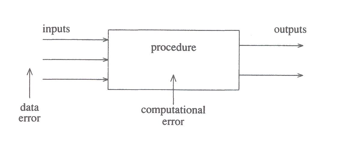
    The errors they do care about they break into two types:

    • Data errors:
      • measurement errors, or
      • errors passed to us by previous calculations.
    • Computational errors:
      • roundoff errors, or
      • truncation errors.
    I might add "output errors" to their Figure 1.7, p. 17:
    

    We don't provide as many decimals as we've obtained, say, in a table. I guess we won't worry about those, either (but, in reality, you need to). It's related to that question "how many digits do I give my answer to?" that students ask.... We don't have a good simple answer.

    The authors make an amusing argument that just because we get error-riddled input doesn't mean that we can be sloppy. "It is best to treat the input values as exact and not make judgments about their accuracy or the morality of computing accurate answers to inaccurate problems." (my emphasis)

    Data errors are propagated through further calculations (error propagation).

    Let $\hat{a}$ be an approximation to datum $a$: then

    $propagated\ data\ error{\equiv}f(\hat{a})-f(a)$

    Then

    $computational\ error{\equiv}{\hat{f}}(\hat{a})-f({\hat{a}})$

    caused by inaccurately computing f. Figure 1.8 is a good one to illustrate these various sources of error, and the discussion:

    

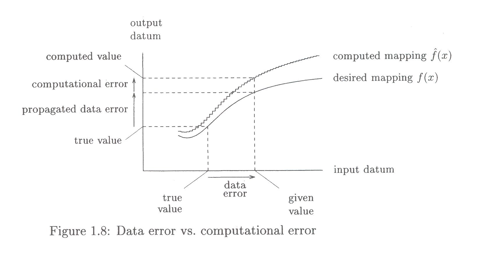
    Let's do an example:

    • suppose we truncate the Taylor series for $e^x$ with only four terms.
    • Plot $f(x)=e^x$ and $f^*(x)=\sum_{n=0}^3\frac{x^n}{n!}$ from $(0,2)$.
    • Suppose we want to compute $e^\sqrt{2}$, but end up computing $e^{1.41}$ instead.
    • Find and illustrate
      1. the error (and relative error) in the datum,
      2. the propogated data error, and
      3. the computational error.

    By the way, notice that if we add the errors we get

    $total\ error{\equiv}{\hat{f}}(\hat{a})-f(a)$

    The total error is made up of the sum of the computational and data propagation errors:

    $total\ error{\equiv}\left(\hat{f}(\hat{a})-f({\hat{a}})\right)+\left(f({\hat{a}})-f(a)\right)$

    One part involves computing the right $f$ with the wrong data, and other involves computing the wrong $f$ on the wrong data!

  • Section 1.4.3: Specifying uncertain quantities

    The authors consider a case where a quantity x does not come to us as a value, but rather as a set of values:

    1.423, 1.399, 1.491, 1.449, 1.480

    How do we proceed?

    Obviously we could do a computation for each value. However then our audience is going to ask us for an answer, and we're going to have a bunch (a set)! They may not be okay with that....

    We could use some statistics to give an answer. We could use the mean of the set of potential values. But we want to avoid losing track that there was some variance in that input (and failing to warn the user at the output end).

    We could treat the value as an interval (from lowest to highest data values), although we'd still have the problem of what to report.

    Let's assume that the true value lies within the data range: we assume that x lies in the interval [1.399,1.491]. So now the question is, what value might we assign to x?

    This section provides a reality check on the term "significant digits" -- "there is no consensus on what this means" -- and they provide an example which illustrates the danger of going with the notion that the least significant digit should be in error by at most 5 units in that place.

    See Figure 1.9:

    

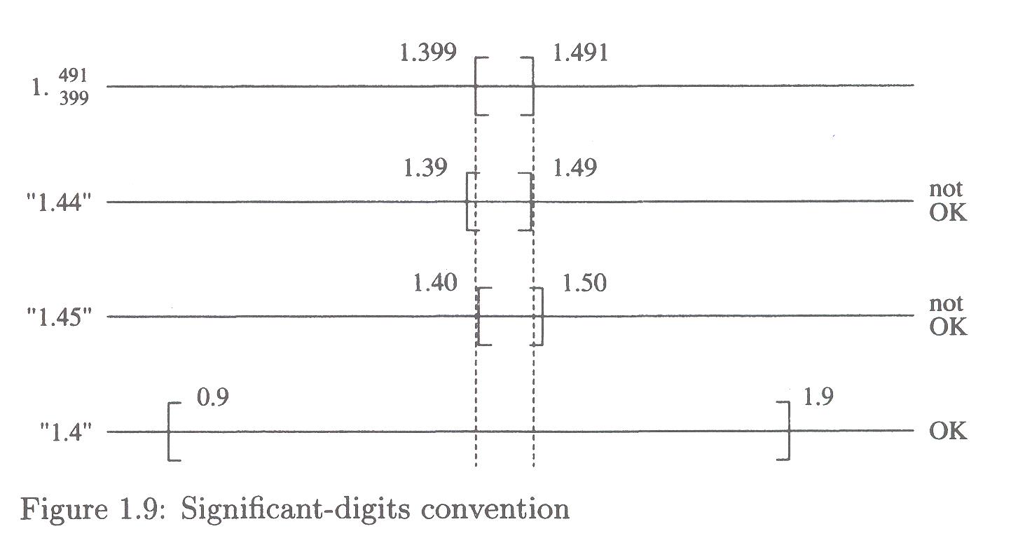
    The question the authors ask (and answer) is this:

    Can you assign a digit to the hundredths place that will not be in error by any more than five hundredths?

  Let's take a look at one problem from the text, #3, p. 20. It's kind of interesting: rather than an ulp, it's asking us for an "ufp". Defining it (may) introduce the floor and ceiling functions, and makes use of logs (and we'll need to understand both in this class).

• Section 1.5: Error Propagation

  The authors give three examples of propagation of errors:

  1. Computation of a side of a triangle from two others.
  2. Roots of Wilkinson's polynomial
  3. Weather prediction (and chaos -- extremely sensitive dependence on initial conditions, p. 24)

  They urge us to keep in mind that "small relative errors in data do not implpy equally small errors in the results." (p. 22)

  They define the condition number of procedure as

  $\frac{|relative\ error\ in\ results|}{|relative\ error\ in\ data|} >> 1$

  Ill-conditioned describes a problem that is sensitive to small changes in initial conditions; well-conditioned describes a problem that is insensitive to small changes in initial conditions.

  • In the first example, a change of .1% in the length of a side leads to a 2.3% error in the calculation of the side of interest.
  • In the second, a microscopic change in a single coefficient (-210 to -210+10^-7) leads to 20% relative errors in the magnitude of some roots -- and they go from real to complex!
  • In weather prediction, small changes in initial conditions can quickly lead to utterly different weather projections. (Authors claim 15 day limit in weather forecasting). There's nothing to do about this system, as it is chaotic.
  There's some good news, however: it's true that in some cases errors don't actually propagate. Data errors to the computation of the square roots as computed by Babylonians don't grow -- they die out. The same root is obtained with a bad starting approximation or a good one. Small errors made up front in choice of the starting value fail to propagate.

  We emphasize that, in this chapter, we are assuming that the procedure itself is carried out exactly (e.g. square roots); the propagated error is simply a consequence of the procedure acting on error (not of how well or poorly the procedure is implemented). That is a matter for section 2.5....

  As examples, the authors consider the ordinary arithmetic operations (which are so-called "binary operations" (taking two inputs).

  The first equation demonstrates the value of one of the equations we looked at last time:

  approximate value = (true value)(1 + relative error)

  Adding a and b, each with a little relative error, we get a sum which is in relative error by

  $(a+b)(1+\epsilon_{a+b}) = a(1+\epsilon_a)+b(1+{\epsilon_b})$

  or

  $(a+b)\epsilon_{a+b} = a\epsilon_a+b{\epsilon_b}$

  so that

  $\epsilon_{a+b} = \frac{a\epsilon_a+b{\epsilon_b}}{a+b}$

  Imagine that there's no relative error in b. Then

  $\epsilon_{a+b}{=}\frac{a{\epsilon_a}}{a+b}$

  and

  $\frac{|\epsilon_{a+b}|}{|{\epsilon_a}|}{=}\frac{|a|}{|a+b|}$

  Question: Under what conditions will this be much much greater (>>) than 1?

  Let's take a look at an example where the errors cause trouble (p. 25 -- "catastrophic cancellation"):

  Interestingly enough, multiplication and division are robust ("well-conditioned") to data errors: performing a similar analysis (#3, p. 28), we have

  $(a*b)(1+\epsilon_{a*b}){=}a(1+\epsilon_a)*b(1+{\epsilon_b})$

  or

  $(1+\epsilon_{a*b}){=}(1+\epsilon_a)*(1+\epsilon_b)$

  so that

  $\epsilon_{a*b}{=}\epsilon_a+\epsilon_b+{\epsilon_a}*{\epsilon_b}$

  Again, imagine that there's no relative error in b. Then

  $\frac{|\epsilon_{a*b}|}{|{\epsilon_a}|}{=}1$

  Another way to simplify the analysis is to assume that the data errors are roughly the same size: then

  $\epsilon_{a*b}{=}2\epsilon_a+{\epsilon_a}^2$

  $\frac{|\epsilon_{a*b}|}{|\epsilon_a|} = 2+\epsilon_a$

  which, again, is not big (assuming small data errors, which is generally the case).
  • Section 1.5.1: Condition number of a unary operation

    So now let's talk about some unary operations (e.g. cosine, rather than the binary operations we just considered). Again, we're going to assume that computations are carried out precisely -- it's just data error propagation we're concerned with at the moment.

    The example our authors consider is one of a function $f({a})$, given data $\hat{a}{=}a(1+{\epsilon_a})$: then

    $f({a})(1+{\epsilon_{f({a})}}){=}f({a(1+{\epsilon_a})})$

    Let's suppose that f is differentiable. If so, then we might make use of the Taylor Series Expansion. I told you earlier to expect it -- here it is, and it will occur over and over again.

    If

    $|a\epsilon_a|<<1$ then we can approximate
    $f({a(1+{\epsilon_a})})=f(a+a{\epsilon_a}){\approx}f({a})+a{\epsilon_a}f'(a)$

    and then

    $f({a})(1+{\epsilon_{f({a})}}){\approx}f({a})+a{\epsilon_a}f'(a)$

    so that

    $\frac{\epsilon_{f({a})}}{\epsilon_a}{\approx}\frac{af'(a)}{f(a)}$

    or

    $\frac{\epsilon_{f({a})}}{\epsilon_a}{\approx}\frac{a}{f(a)}f'(a)$

    which our authors call the relative derivative of $f({x})$ at $a$, and the condition number of $f({x})$ at $a$ is the absolute value of the relative derivative of $f({x})$ at $a$.

    In particular, this works better and better as $\epsilon_a\to{0}$.

    We can say, in particular, that the condition is directly proportional to the derivative, and to the size of a; it's inversely proportional to the size of $f({a})$.

    Examples: compute the relative derivative of

    • $f(x){=}e^x$
    • $f(x){=}\ln(x)$
    • $f(x){=}\sin(x)$
    How do these two differ in their condition?

  • Section 1.5.2: Interval analysis

    I've got to say that I'm not a huge fan of interval analysis, in general. For example, in a problem exhibiting chaos, intervals can go haywire (source).

    Interval analysis is well-behaved when the functions involved are monotonic (increasing or decreasing). But, as the authors illustrate, two different expressions for the same quantity can yield different intervals.

    Think about the interval $[0,-{\pi}]$ for $\sin(x)$. If you just check the endpoints, you get the single point 0.

    And if a function is discontinuous, all hell can break loose!

Floor[Log[10, Abs[17.5]]]
Floor[Log[10, Abs[-.0235]]]

10^Floor[Log[10, Abs[17.5]]]
10^Floor[Log[10, Abs[-.0235]]]

If not, and we must use 1.4, then another user would assume that we only know the 4 in the tenths place to within five units, and you can see what happens to the actual uncertainty -- it expands grossly, to the interval (0.9,1.9).

The speed of light in a vacuum.















































When

and, in particular, when $a+b{\approx}{0}$, i.e. when

Symmetrically, subtraction will suffer the problem when a and b are approximately equal.

TableRow[true_, approximate_] :=
 {error[true, approximate], 
  relativeError[true, approximate], 
  decimalsOfAccuracy[error[true, approximate]],
  digitsOfAccuracy[relativeError[true, approximate]]}
TableRow[1.2345, 1.2346]
TableRow[9.2345, 9.2346]
TableRow[10.2345, 10.2346]
TableRow[100.2345, 100.2346]
TableRow[1000.2345, 1000.2346]

a = 100;
astar = 100.1;
b = 101;
TableRow[true_, approximate_] :=
 {true, approximate, 
  100* relativeError[true, approximate]}
TableRow[a, astar]
TableRow[b - a, b - astar]
TableRow[(b - a)^2, (b - astar)^2]
TableRow[4.*a* b* Sin[Pi/360]^2, 4.*astar* b* Sin[Pi/360]^2]
TableRow[(b - a)^2 + 4.*a* b* Sin[Pi/360]^2, (b - astar)^2 + 
  4.*astar *b *Sin[Pi/360]^2]
TableRow[Sqrt[(b - a)^2 + 4.*a* b* Sin[Pi/360]^2], 
 Sqrt[(b - astar)^2 + 4.*astar* b *Sin[Pi/360]^2]]
TableRow[Sqrt[b^2 + a^2 - 2.*a* b* Cos[Pi/180]], 
 Sqrt[b^2 + astar^2 - 2.*astar* b* Cos[Pi/180]]]

cond[f_, a_] := Abs[f'[a]*a/f[a]]
cond[Exp, x]
cond[Log, x]
g[x_] = cond[Sin, x]
Plot[g[x], {x, 0, Pi/2}]