- Final Exam: 10:10, Thursday, May 4.
- Your integration homework is returned. Comments:
- p. 281, #1: they'd intended a composite scheme (so you have to do more than one panel). No points off, however: the important thing is to know how to do each scheme, number one: but you also have to know how to handle a bunch of panels strung together....
- p. 281, #2: Joey
- p. 281, #15d: Trey
- p. 293, #1: Lauren
- p. 293, #4a: Alyssa
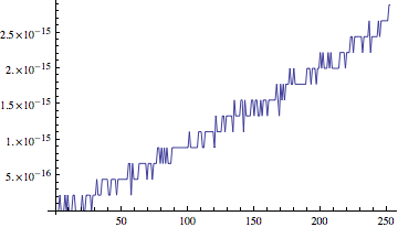
- Any questions on project 2? I've received several! One
important little details is that it appears to me that the
formula they use on p. 203 is in error. I've got some
Mathematica code to illustrate that.
I also went ahead and used lisp to implement the plotting routine as plotter, and as adaptive quadrature method.
- Your homework, on DEs, is due this week, Friday am. So get your project done (due Thursday) first, but don't forget your homework.
- So we've seen Euler's method in action,
\[
U(t_{n+1}) = U(t_{n})+ h U'(t_{n}) + \frac{h^2}{2}U''(\xi_{n}) \approx U(t_{n})+ h U'(t_{n}) = U(t_{n})+ h f(t_n,U(t_n))
\]
and we now know what kind of errors to expect. Let's predict the error
of Euler applied to our exponential spline -- i.e., we want to estimate
$e^x$ on the interval [0,1]; so our differential equation is
\[
Y'(t)=Y(t)
\]
with initial condition
\[
Y(0)=1
\]
For which we want a solution on [0,1].
Questions:
- Is this DE's RHS Lipschitz? What's $L$ for the IVP problem?
- What's the bound for the second derivative on this interval?
- What's the bound on the global error we'd expect at 1 (ignoring rounding or data errors)?
- Let's check!
Before we do that, however, a brief reminder that Euler's method can be used very generally: for a system, and for higher-order ODEs:
- An example system (lynx and hares)
- An example 2nd-order ODE (harmonic oscillator)
\[ |y(t_i)-u_i| \le \frac{1}{L}\left(\frac{hM}{2}+\frac{\delta}{h}\right) \left[e^{L(ih)}-1\right] + |\delta_0|e^{L(ih)} \]
The neat thing is that we can arrive at an optimal $h$ to reduce the error at the end of interval, when $i=N$, to below some given small error target $\epsilon$:
\[ |y(b)-u_N| \le \frac{1}{L}\left(\frac{hM}{2}+\frac{\delta}{h}\right) \left[e^{L(b-a)}-1\right] + |\delta_0|e^{L(b-a)} < \epsilon \]
provided we can bound the second derivative and the rounding errors:
$h=\sqrt{\frac{2\delta}{M}}$ For our machine, we have perhaps $\delta=10^{-17}$, and for this problem we have $M=e$. So our expectation is that $h=\sqrt{\frac{2 \times 10^{-17}}{e}}\approx 2.712E-9$.
- Euler's method is an example of a Taylor method -- it's the first
in a series (we might call it "Taylor-1"). So it's our introduction to
Taylor methods, which we can think of as generalizations of Euler's
method.
In particular, we generalize the formula on p. 323,
$y_{n+1}=y_{n}+hf(t_{n},y_n)$ to the more general formula
$y_{n+1}=y_{n}+h\phi(t_{n},y_n;h)$ Note the parameter $h$ in the $\phi$ function: $\phi$ will generally be a function of $h$. We think of it as an improved derivative calculation -- but it's just based on information at the $n^{th}$ time step. So these are "first-order" methods -- they take into account only the preceeding time step.
- As we saw last time, Euler can be derived as the tangent line
approximation to solution of the ODE. We could just as easily pass a
quadratic through the point $(t_i,y(t_i))$ that interpolates the slope
and the curvature (2nd derivative) as well (Figure 8.19, p. 340). This
is the idea behind Taylor-2:
\[ U(t_{n+1}) = U(t_{n})+ h U'(t_{n}) + \frac{h^2}{2}U''(t_{n})+ \frac{h^3}{3!}U'''(\xi_{n}) \]
and we throw away the $O(h^3)$ stuff (that's the local truncation error). Then we figure out a way to write that second derivative....
And so on! That's the idea of the higher-order Taylor methods.
The name "Taylor-2" suggests that we can simply derive these methods from Taylor's theorem, and that's what we saw last time. We simply include the second-derivative info, and we obtained
\[ U''(t_n) = \frac{\partial f}{\partial t}\bigg\rvert_{t_n,y_n}+ \frac{\partial f}{\partial y}\bigg\rvert_{t_n,y_n}f(t_n,y_n) \]
So, in this case, \[ \phi(t_n,y_n;h) = f(t_n,y_n) + \frac{h}{2}\left(\frac{\partial f}{\partial t}\bigg\rvert_{t_n,y_n}+ \frac{\partial f}{\partial y}\bigg\rvert_{t_n,y_n}f(t_n,y_n)\right) \]
That is, $\phi$ is Euler's step (Taylor-1), with an adjustment for the concavity of the function (represented by the second derivative).
Examples:
- Using successively higher Taylor Methods (computational version). We'll try out an example that our authors suggest, and then our favorite ($e^x$).
- Using successively higher Taylor Methods
This code is not optimized for approximation, but shows the dependence of each successive step on $h$ (values are defined recursively).
If you increase $n$ you will eventually exceed the recursion limit of Mathematica.
A small change in how the $w$ values are computed makes it efficient for calculation.
- Computer problem #1, p. 344 (I'm not sure why the authors suggest the step-size control that they do -- they seem to be off by a power of $h$, and a derivative.)
- A modification of that code to do other examples, e.g. Example 8.10, p. 340
- Using successively higher Taylor Methods (computational version). We'll try out an example that our authors suggest, and then our favorite ($e^x$).
Now we go about eliminating the derivatives, creating Runge-Kutta Methods. They are based on a clever observation about the multivariate Taylor series expansion.
- We start with an illustration of how we might improve on Euler's
method, by replacing it by Runge's midpoint. So check out 8.5.1,
p. 346, and Figure 8.20 in particular.
- Alternatively we might replace it with Runge's trapezoidal
method (Figure 8.21).
- But ideally, we'll figure out how to replace a method (such as
Taylor-2) with something that gives us the same order, but without
computing derivatives. That's the job of RK-2.
- The derivation involves Taylor series expansions of functions of
two variables.
- How do we think about Taylor series geometrically for functions of two variables?
- Now let's derive each, and show how they're of the same order as Taylor-2.
- Let's compare other estimates on Example 8.11:
Euler's Taylor-2 Runge Midpoint Runga Trapezoidal 1.583 - Let's have a look.
- You might be thinking "why not just do two half-steps of Euler?"
I mean, we're doing more work to get an RK-2. Why do you think that RK-2 is better than simply doing Euler twice as often? It's about the same amount of work....
- RK-4 involves matching more derivatives: see p. 349 for equations,
and geometry.
- Many folks' go-to ODE solver is RK-4, with step-size
control. In the following Mathematica code, I adapt the
step-size control we used with Taylor to the RK-4 in some
sensible way.