- Your revisions and homeworks are returned. Courtney did a really nice job of using Mathematica to solve each and every problem. Her code was a lot better than mine....:( ...:)
- Any questions on project 2?
- Your integration homework is due.
- I have assigned a new homework, on DEs. This will be due next week, Friday am. So get your project done first, but don't forget your homework.
- So we've seen Euler's method in action,
\[
U(t_{n+1}) = U(t_{n})+ h U'(t_{n}) + \frac{h^2}{2}U''(\xi_{n}) \approx U(t_{n})+ h U'(t_{n}) = U(t_{n})+ h f(t_n,U(t_n))
\]
and we now know what kind of errors to expect. Let's predict the error
of Euler applied to our exponential spline -- i.e., we want to estimate
$e^x$ on the interval [0,1]; so our differential equation is
\[
Y'(t)=Y(t)
\]
with initial condition
\[
Y(0)=1
\]
For which we want a solution on [0,1].
Questions:
- Is this DE's RHS Lipschitz? What's $L$ for the IVP problem?
- What's the bound for the second derivative on this interval?
- What's the bound on the global error we'd expect at 1 (ignoring rounding or data errors)?
- Let's check!
Before we do that, however, a brief reminder that Euler's method can be used very generally: for a system, and for higher-order ODEs:
- An example system (lynx and hares)
- An example 2nd-order ODE (harmonic oscillator)
\[ |y(t_i)-u_i| \le \frac{1}{L}\left(\frac{hM}{2}+\frac{\delta}{h}\right) \left[e^{L(ih)}-1\right] + |\delta_0|e^{L(ih)} \]
The neat thing is that we can arrive at an optimal $h$ to reduce the error at the end of interval, when $i=N$, to below some given small error target $\epsilon$:
\[ |y(b)-u_N| \le \frac{1}{L}\left(\frac{hM}{2}+\frac{\delta}{h}\right) \left[e^{L(b-a)}-1\right] + |\delta_0|e^{L(b-a)} < \epsilon \]
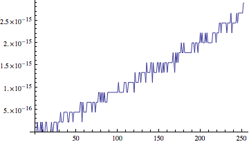
provided we can bound the second derivative and the rounding errors:
$h=\sqrt{\frac{2\delta}{M}}$ For our machine, we have perhaps $\delta=10^{-17}$, and for this problem we have $M=e$. So our expectation is that $h=\sqrt{\frac{2 \times 10^{-17}}{e}}\approx 2.712E-9$.
- Euler's method is an example of a Taylor method -- it's the first
in a series (we might call it "Taylor-1"). So it's our introduction to
Taylor methods, which we can think of as generalizations of Euler's
method.
In particular, we generalize the formula on p. 323,
$y_{n+1}=y_{n}+hf(t_{n},y_n)$ to the more general formula
$y_{n+1}=y_{n}+h\phi(t_{n},y_n;h)$ Note the parameter $h$ in the $\phi$ function: $\phi$ will generally be a function of $h$. We think of it as an improved derivative calculation -- but it's just based on information at the $n^{th}$ time step. So these are "first-order" methods -- they take into account only the preceeding time step.
- As we saw last time, Euler can be derived as the tangent line
approximation to solution of the ODE. We could just as easily pass a
quadratic through the point $(t_i,y(t_i))$ that interpolates the slope
and the curvature (2nd derivative) as well (Figure 8.19, p. 340). This
is the idea behind Taylor-2:
\[ U(t_{n+1}) = U(t_{n})+ h U'(t_{n}) + \frac{h^2}{2}U''(t_{n})+ \frac{h^3}{3!}U'''(\xi_{n}) \]
and we throw away the $O(h^3)$ stuff (that's the local truncation error). Then we figure out a way to write that second derivative....
And so on! That's the idea of the higher-order Taylor methods.
The name "Taylor-2" suggests that we can simply derive these methods from Taylor's theorem, and that's what we saw last time. We simply include the second-derivative info, and we obtained
\[ U''(t_n) = \frac{\partial f}{\partial t}\bigg\rvert_{t_n,y_n}+ \frac{\partial f}{\partial y}\bigg\rvert_{t_n,y_n}f(t_n,y_n) \]
So, in this case, \[ \phi(t_n,y_n;h) = f(t_n,y_n) + \frac{h}{2}\left(\frac{\partial f}{\partial t}\bigg\rvert_{t_n,y_n}+ \frac{\partial f}{\partial y}\bigg\rvert_{t_n,y_n}f(t_n,y_n)\right) \]
That is, $\phi$ is Euler's step (Taylor-1), with an adjustment for the concavity of the function (represented by the second derivative).
Examples:
- Using successively higher Taylor Methods (computational version). We'll try out an example that our authors suggest, and then our favorite ($e^x$).
- Using successively higher Taylor Methods
This code is not optimized for approximation, but shows the dependence of each successive step on $h$ (values are defined recursively).
If you increase $n$ you will eventually exceed the recursion limit of Mathematica.
A small change in how the $w$ values are computed makes it efficient for calculation.
- Computer problem #1, p. 344 (I'm not sure why the authors suggest the step-size control that they do -- they seem to be off by a power of $h$, and a derivative.)
- A modification of that code to do other examples, e.g. Example 8.10, p. 340
- Using successively higher Taylor Methods (computational version). We'll try out an example that our authors suggest, and then our favorite ($e^x$).
Now we go about eliminating the derivatives, creating Runge-Kutta Methods. They are based on a clever observation about the multivariate Taylor series expansion.
- We start with an illustration of how we might improve on Euler's
method, by replacing it by Runge's midpoint. So check out 8.5.1,
p. 346, and Figure 8.20 in particular.
- Alternatively we might replace it with Runge's trapezoidal
method (Figure 8.21).
Let's compare other estimates on Example 8.11:
Euler's Taylor-2 Runge Midpoint Runga Trapezoidal 1.583 - But ideally, we'll figure out how to replace a method (such as
Taylor-2) with something that gives us the same order, but without
computing derivatives. That's the job of RK-2.
- The derivation involves Taylor series expansions of functions of
two variables.
- How do we think about Taylor series geometrically for functions of two variables?
- You might be thinking "why not just do two half-steps of Euler?" I
mean, we're doing more work to get an RK-2. Why do you think that RK-2
is better than simply doing Euler twice as often? It's about the same
amount of work....
- Many folks go with an RK-4, with step-size control. I am trying to
adapt the step-size control we used with Taylor to the RK-4 in some
sensible way (but not having much luck yet). If we have a little time
left, maybe we can talk about that issue....
- Applications