- There was a great talk
last night, by the author of Code Girls, Liza Mundy.
Alyssa, Rachel, and Jacob (at least) were there -- what did you think?
- There is a departmental lunch -- today! Come on up, and
enjoy lunch on us. 11:30-1:00, fourth floor. Come one and all!
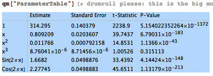
- Your Keeling models are returned. This is exactly the same
sort of analysis you'll want to perform on your Togo
temperature data, so I hope that it has you ramped up for that.
(By the way, you could even use the decimal dates of the Keeling
model for the months of the Togolese data. The Togolese months
overlap those of the Keeling data.)
Remember UPCE: One thing I want to see more of is interpretation and evaluation: what do the parameter tables tell us? What are the residuals saying?
We need to learn to give voice to our data. It's speaking, but is anyone listening? If data falls in a forest, does anyone hear?
Then we'll try to sing a song that sounds like the data. Math modelers are like people trying to imitate bird song in the forest. We want to find a way to imitate the data; and if we can ultimately call in the right bird with our song, we're successful.
Joey heard something really interesting!
Let's see if we can describe what he heard....
- You have an assignment due today (your review of your new
city's mini-project report, and your own -- and partners); and
I've postponed your "small assignment" about Ad expenditures
until Monday. Any questions about that?
Jacob asked a good question about confidence intervals for linearized models: when you cast your data over into "log space", we compute confidence intervals for the parameters.
When we transform the parameters back (e.g. $a=e^\alpha$) do we simply transform the confidence intervals in the same way? Those are just bounds on the true value of $a$, so it seems reasonable.
The probability remains the same for the back-transformed intervals, but when you log or exp-transform something, what was previously symmetric loses its symmetry. CIs are symmetric. So the parameter value, which was right in the middle of the transformed CIs, will not be in the middle of the back-transformed intervals.
Imagine, for example, that the CI for $\alpha$ were $2 \pm 1$. If we exponentiate that, we get a back-transformed interval for $a$ of $(e^1,e^3) \approx (2.72,20.09)$, with the parameter estimate at $a=7.39$ (leaning to the left).
If we perform non-linear regression, we'll get a symmetric confidence interval!
So let's take a quick look at the Ad Expenditures file, which I've modified slightly to add a purely non-linear regression to compare with our linearization. There are some surprising results!
- A couple of words on parsimony: adding the cubic term to
the Keeling model didn't really achieve anything (other than a very
slight improvement in $R^2$) -- it wasn't "worth the cost" in some
sense -- KISS, and Occam's razor, and all that.

- So last night I got an email from the American Journal of Climate Change, soliciting manuscripts for a special issue on "Climate Dynamics", with a submission due date of May 17th. This is our journal, and this is our special issue!
- We began study of non-linear regression, and I started
with Newton's method, (which some of you will have seen
before, and others of you may not have seen).
The key to non-linear regression is linear regression! That may seem odd, but I will mention again that frequently in mathematics we often cast a problem from the non-linear world over to where we obtain a linear problem, then bring that solution back (and hope for the best).
In the case of the linearizations we have done, we only did this "casting" trick once -- then we were done. In the case of non-linear regression, we will do it multiple times (iteratively), hoping for continual improvement.
After I described Newton's method, I went through an actual example with you, from my non-linear regression derivation page.
Let's take a moment to play with Newton's method a bit, using this code.
We'll begin by moving on from Newton's method, to show how non-linear regression is cast into the linear world; and then we'll have a look at cadavers (well, figuratively speaking!:): here's the Mathematica file.
As we think about modeling the onset of rigor mortis, we might start with the Bestiary of functions, from Ben Bolker's Ecological Models and Data in R. Do we hear any songs that sound like our data? If not, we may have to go off-road, to mix metaphors....
