Section12SIR Model and Differential Equations¶ permalink

Subsection12.1InsightMaker¶ permalink

A simple model of infectious disease can be created in a visual and, dare-I-say, even enjoyable way using a "free" website called InsightMaker. These "compartmental" models allow one to build models visually, by creating "stocks" and "flows" and parameters, etc., and getting them connected up the way you want. Then you can "simulate" the dynamics, illustrating the facets you want with time-series, or scatterplots, or what-have-you.

Anyway, this is all the commercial message you're going to get, but it's a nice piece of software that gently introduces one to modeling dynamical systems.

They also have a lot of nice demos on hand, created by individuals willing to share, so I was able to pick up an SIR model ("clone" it) from another user, and we've been playing with that.

So, once we're done building the model in InsightMaker, what have we actually done? We've built a system of differential equations, which we can solve using any standard mathematical software (e.g. Mathematica).

I want to take a look at the SIR from the differential equation standpoint now, and reduce the system we've been studying down to its sleekest, most elegant form. We do so, however, at the cost of some mathematical analysis.

Subsection12.2The SIR Model¶ permalink

In the end, once all the flows have been set out, the parameters described and their ranges set, we watch as the populations in the "stocks" go through their motions. And we wonder "what kinds of dynamic behaviors are possible?"

The visual elements of InsightMaker are translated into equations, called differential equations, that are then solved (numerically) by turning them into difference equations (discrete versions of the continuous differential equations).

The flows that we've established, represented in this diagram,

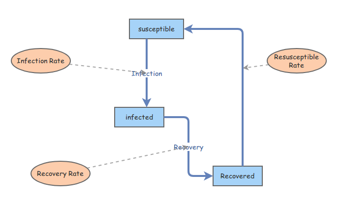are converted into the following system of equations, which represent the populations at the next moment, a timestep \(\Delta t\) later:

\begin{equation*} \begin{array}{l} \displaystyle S(t+\Delta t) = S(t) + (-\alpha S(t)I(t) + \gamma R(t))\Delta t \cr I(t+\Delta t) = I(t) + ( \alpha S(t)I(t) - \beta I(t))\Delta t \cr R(t+\Delta t) = R(t) + (-\gamma R(t) + \beta I(t))\Delta t \end{array} \end{equation*} where \(\alpha\) is the infection "rate", \(\beta\) is the recovery rate, and \(\gamma\) is the resusceptible rate. Notice that I put the infectivity "rate" in quotes: there's an issue that we're going to discuss in a moment.

Now divide each side by \(\Delta t\), and we've got \begin{equation*} \begin{array}{l} \displaystyle \frac{S(t+\Delta t)-S(t)}{\Delta t} =-\alpha S(t)I(t) + \gamma R(t) \cr \frac{I(t+\Delta t)-I(t)}{\Delta t} = \alpha S(t)I(t) - \beta I(t) \cr \frac{R(t+\Delta t)-R(t)}{\Delta t} = -\gamma R(t) + \beta I(t) \end{array} \end{equation*}

Then take a limit as \(\Delta t \to 0\), and we finally have our system of differential equations: \begin{equation*} \begin{array}{l} \displaystyle S'(t) =-\alpha S(t)I(t) + \gamma R(t) \cr I'(t) = \alpha S(t)I(t) - \beta I(t) \cr R'(t) = -\gamma R(t) + \beta I(t) \end{array} \end{equation*}

Okay: if you scaled the sub-populations by multiplying each by 100, should that change the dynamics? Or would everything proceed the same, just on a 100-fold larger scale? I would think that everything would look the same, just on a 100-fold larger scale. However, if you scale each sub-population by 100, the dynamics change. That's because of the "bi-linear" term \(S(t)I(t)\): we would have to divide \(\alpha\) by 100 to keep the same dynamics. That's a problem, and one which shows that \(\alpha\) is not the rate that we expect. I'll handle that problem in a moment.

First, let's consider the total population, \(N(t)=S(t)+I(t)+R(t)\). It turns out that \(N(t)\) is actually constant, since \begin{equation*} \frac{dN(t)}{dt}=\frac{d}{dt}(S(t)+I(t)+R(t))=0 \end{equation*} (just add all the right-hand sides of the system of equations to see that they cancel each other).

This just says that no one is lost to the system - they stay in one population or the other, and no people are created or destroyed. \(N(t)\) called a conserved quantity. Since \(N(t)\) is actually constant, let's just call it \(N\).

If we divide all the populations by \(N\), then they're turned into proportions, which sum to 1.

Now back to the problem mentioned just a moment ago. Actually, the interaction term, which models the infection flow, has the wrong units if we think of \(\alpha\) as a rate (the rates have units of \(\frac{1}{time}\): however, if we change that flow from \begin{equation*}\alpha S(t)I(t)\end{equation*} to \begin{equation*}\alpha S(t)\frac{I(t)}{N}\end{equation*} then we're okay. So let's do that, and then \(\alpha\) is back to the rate that we think it is.

It also changes how we think about the interaction. We still have a bi-linear relationship: if you double the infected population, you'll double the number of infected susceptibles; and if you double the number of susceptibles, you'll double the number of infected susceptibles. But it now has the units of \(\frac{people}{time}\), which is then multiplied by \(\Delta t\) to turn that flow into a flow of \(people\)!

Think of \(\frac{I(t)}{N}\) as the proportional to the probability that a susceptible will bump into an infected person.

Okay: now we've got a new system, where every sub-population has been scaled by dividing by \(N\):

\begin{equation*} \begin{array}{l} \displaystyle s'(t) =-\alpha s(t)i(t) + \gamma r(t) \cr i'(t) = \alpha s(t)i(t) - \beta i(t) \cr r'(t) = -\gamma r(t) + \beta i(t) \end{array} \end{equation*}

Now, for our final trick, we divide each side of each equation by \(\alpha\):

\begin{equation*} \begin{array}{l} \displaystyle \frac{ds}{\alpha dt} = -s(t)i(t) + \frac{\gamma}{\alpha} r(t) \cr \frac{di}{\alpha dt} = s(t)i(t) - \frac{\beta}{\alpha} i(t) \cr \frac{dr}{\alpha dt} = -\frac{\gamma}{\alpha} r(t) + \frac{\beta}{\alpha} i(t) \end{array} \end{equation*}

and we define new parameters

\begin{equation*} \begin{array}{l} \displaystyle \frac{ds}{\alpha dt} = -s(t)i(t) + \mu r(t) \cr \frac{di}{\alpha dt} = s(t)i(t) - \lambda i(t) \cr \frac{dr}{\alpha dt} = -\mu r(t) + \lambda i(t) \end{array} \end{equation*} where \(\lambda=\frac{\beta}{\alpha}\), and \(\mu=\frac{\gamma}{\alpha}\). These are relative rates, rates relative to \(\alpha\), and the only two parameters left in our model. As we play with these parameters, we'll see all the dynamics possible in this system.

If we now rescale time, as \(\tau=\alpha t\); then, by the chain rule,

\begin{equation*}\frac{ds}{\alpha dt}=\frac{ds}{\alpha d\tau}\frac{d\tau}{dt}=\frac{ds}{\alpha d\tau}\alpha=\frac{ds}{d\tau}\end{equation*}

What does this rescaling of time mean? Let's consider an example, where the infection rate is \(\alpha=1/100/day\). Then if \(\tau=1\), then \(\alpha t=1\), so \(t=100\) days. So time is relative to the disease's infection rate.

What this tells us is that the qualitative picture of two diseases with a different values of \(\alpha\) will look qualitatively the same dynamically, provided the other rate ratios are equal.

So the simplest, sleekest equations are these:

\begin{equation*} \begin{array}{l} \displaystyle \frac{ds}{d\tau} = -s(\tau)i(\tau) + \mu r(\tau) \cr \frac{di}{d\tau} = s(\tau)i(\tau) - \lambda i(\tau) \cr \frac{dr}{d\tau} = -\mu r(\tau) + \lambda i(\tau) \end{array} \end{equation*}

In the end, there's not a lot that can happen: either the infection dies out, or it becomes endemic, and we reach a "steady state", wherein each of the three populations tends towards an asymptotically stable value.

To find the steady state, you need to find a set \((s^*,i^*,r^*)\) which makes each right-hand side of the system of equations above exactly zero - which means that the sub-populations are not changing in time (their derivatives are zero). That's called a fixed point of the system. Then the question becomes "Is it stable?": that is, if we push the system away from the fixed point, does it come back, or fly away?

The parameter \(\lambda\) is critical. It turns out that if \(\lambda\) (which is the ratio of recovery-to-infection rates) is greater than 1, then the infection will die out; if it is less than 1, then the infection will become endemic - remain forever in the population. So it's really important.