Day 37 in Mat329

• Your 15.8 and 15.9 homework is due today. How is that going?

• Your next homework is due Friday (16.1).

We now consider vector-valued functions in multivariate space. We've seen these before, however: if we have a multivariate function $f$ which is differentiable, then it has a gradient at every point, pointing to higher values of $f$.

This is an important example: a gradient field.

• Not all vector fields are gradient fields, however: in general, we might think of a vector field F as ${\bf{F}}=\langle P(x,y),Q(x,y) \rangle$.

  Q: Is the vector field of Example 1 a gradient field?

  If F is a gradient field, then it is called a conservative vector field (and $f$ its potential function).

• Examples:
  • Jared Antrobus (former NKU student and now PhD student in mathematics at UK) provided some Mathematica code that gives insight into the gradient field, and its relationship to maxes and mins: Classify3DGradientField.nb

    This code plots the functions, with maxes and mins, but adds in the contour lines, and also the gradient lines.

    Let's use this to take a look at Example 6, p. 1084.

    

  • #11-14, 1085
  • #1
  • #2
  • #21
  • #25

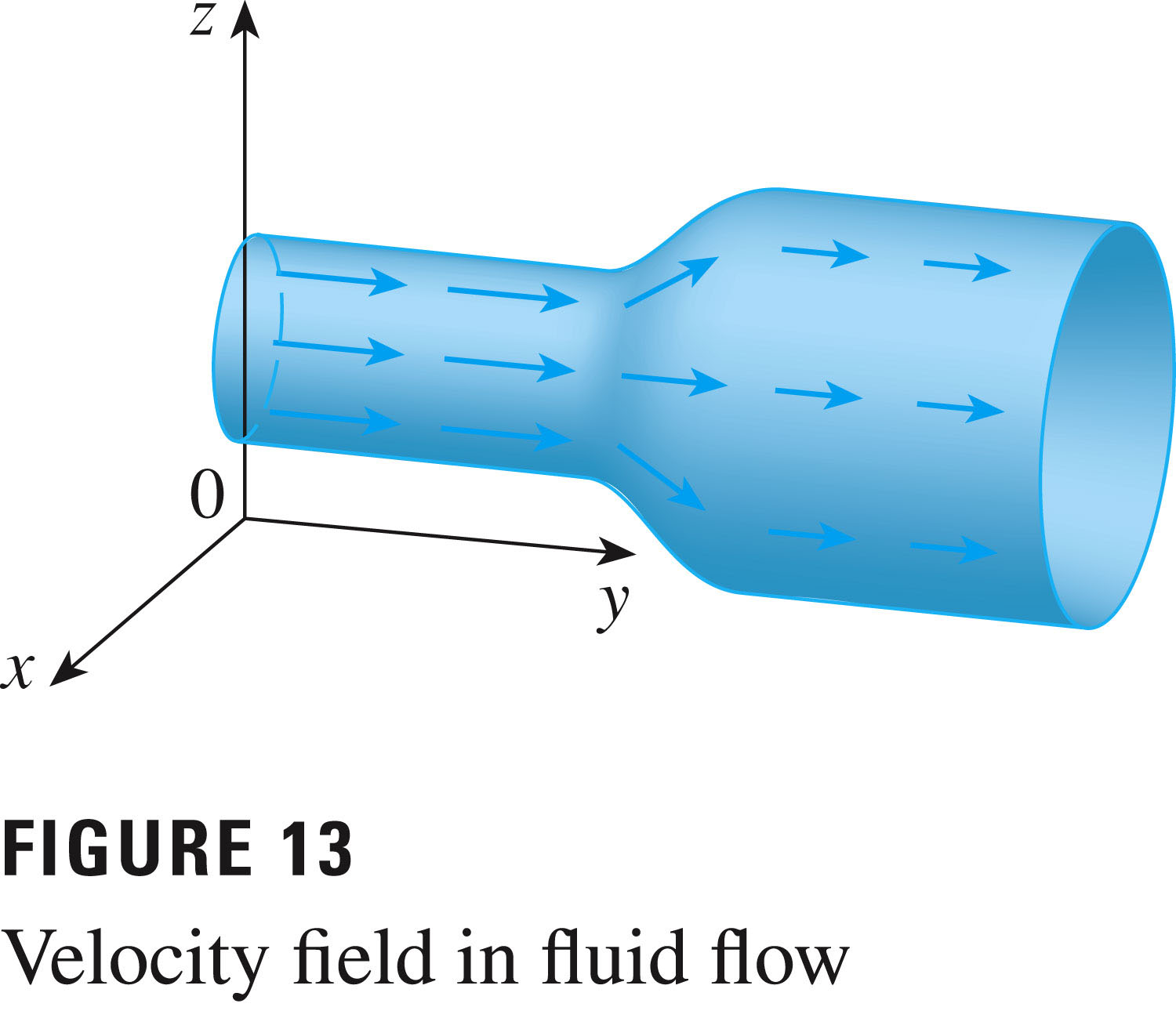
    For the next two problems, we're talking about velocity fields:

    

  • #34:

    StreamPlot[{x y - 2, y^2 - 10}, {x, 0, 4}, {y, 0, 4}, StreamStyle -> ColorData[1][3]]

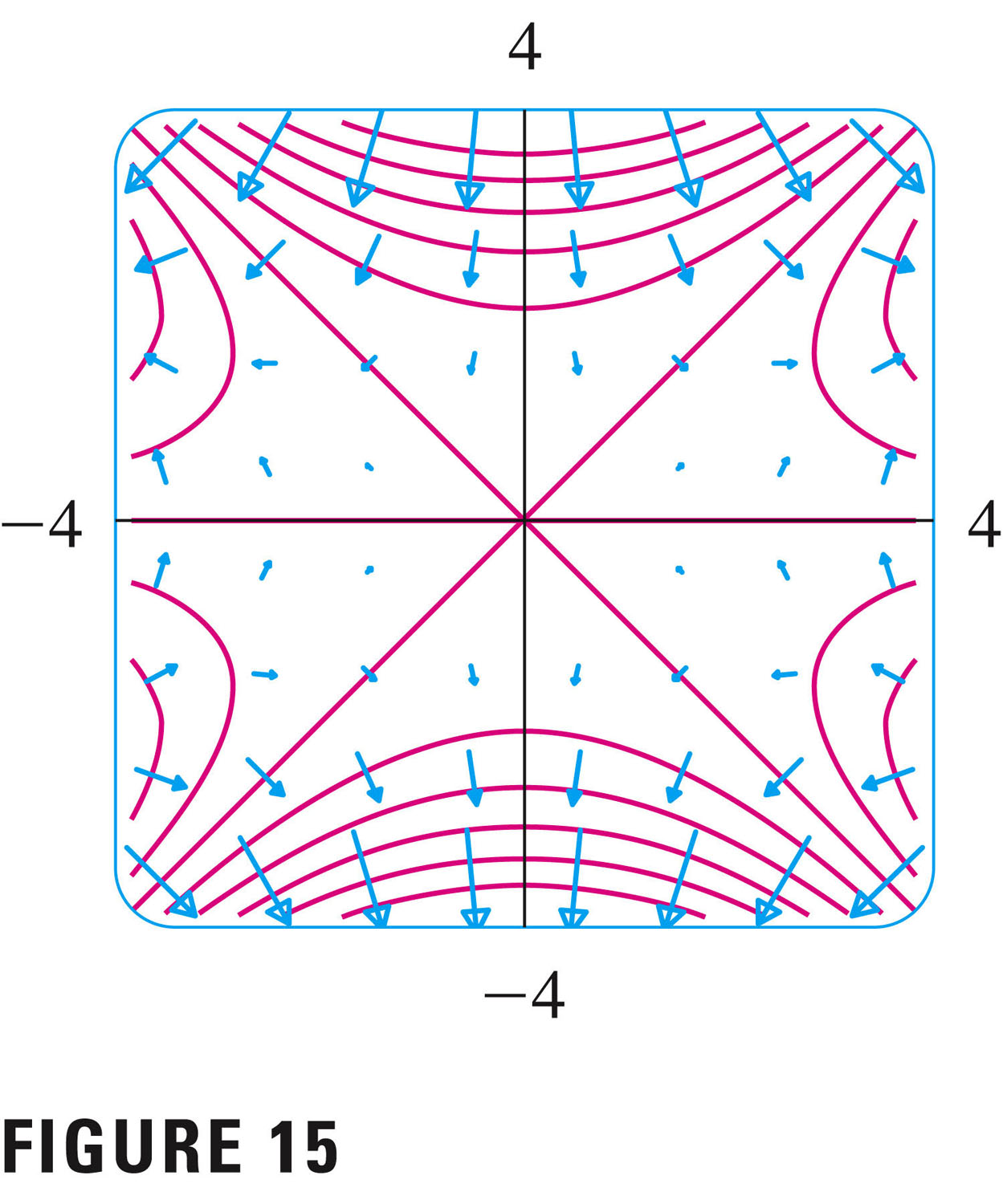
  • #35 -- I've been plotting streamlines, so let's talk about them!:)

    StreamPlot[{x , -y}, {x, -4, 4}, {y, -4, 4}, StreamStyle -> ColorData[1][3]]

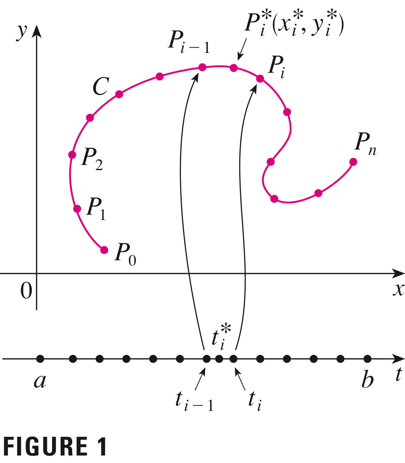
• The line integral of $f$ along $C$ is \[ \int_{C} f(x,y)ds = \lim_{n \to \infty}\sum_{i=1}^{n}f(x_i^*,y_i^*) \Delta s \]
  

• If $f$ is continuous, then \[ \int_{C} f(x,y)ds = \int_{a}^{b} f(x(t),y(t)) {\sqrt{\left(\frac{dx}{dt} \right)^2 + \left(\frac{dy}{dt} \right)^2 }} dt \] and this is independent of the parameterization $(x(t),y(t))$ (provided the curve is traversed just once) as $t$ increases from $a$ to $b$.

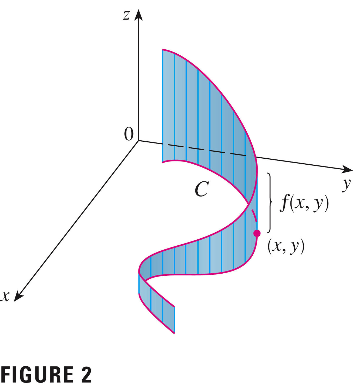
  We can think of this as an area, per Figure 2 (if $f$ is positive):

  

  Although with $f(x,y)=1$ we can also think of this as the length of the curve. Note: we think of $dt$ as positive (and it is, because we've specified the orientation). But if we reverse the orientation, we'd need to "reverse $dt$" as well.

• Rather than look at line integrals along the curve $C$, with differential $ds$, we could integrate components along the $x$ and $y$ directions: line integrals of $f$ along $C$ with respect to $x$ and $y$ are \[ \int_{C} f(x,y)dx = \int_{a}^{b} f(x(t),y(t)) x^{'}(t) dt \] and \[ \int_{C} f(x,y)dy = \int_{a}^{b} f(x(t),y(t)) y^{'}(t) dt \]
• Let's look at Example 4 first, then take on #8, p. 1096. Example 4, p. 1091,
  • raises the issue of orientation;
  • illustrates two different strategies of parameterization;
  • telegraphs a topic of section 16.3: path independence of line integrals.
  • We can think of re-think this one as a vector field problem.

• Examples:
  • #8, p. 1096 (with lots of extra detail)
  • #12 (3-d versions of all of this is no big deal)

• Now we want to extend our line integrals to vector fields.

  Let ${\bf{F}}$ be a continuous vector field defined on a smooth curve $C$ traced out by the vector function ${\bf{r}}(t)$, $a \le t \le b$. Then the line integral of ${\bf{F}}$ along $C$ is \[ \int_{C} {\bf{F}}({\bf{r}}(t)) \cdot d{\bf{r}} = \int_{C} {\bf{F}}({\bf{r}}(t)) \cdot {\bf{r}}^{'}(t) dt = \int_{C} {\bf{F}} \cdot {\bf{T}} ds \] where ${\bf{T}}$ is the tangent vector (the component of velocity in the direction tangential to the motion).

  If vector field ${\bf{F}}=P\hat{i}+Q\hat{j}+R\hat{k}$=$\langle P,Q,R \rangle$, then we can break the integral into three: \[ \int_{C} {\bf{F}} \cdot d{\bf{r}} = \int_{C} Pdx + Qdy + Rdz \] With my parentheses fascination, you can be sure that I'd like to put parentheses around that last integrand: $\int_{C} (Pdx + Qdy + Rdz)$ -- just to emphasize that the integration is over all....

  Examples:

  • #32
  • I want to build up to #52.