 and Mark
L. Wilson
Andrew Long and Mark
L. Wilson
Prior to 1991, raccoon rabies was unknown in the state of Connecticut, USA. In that year, an epizootic of raccoon rabies began its passage across the state, proceeding generally from the west to the east. Wilson, et al.[8] reported on the epizootic using data on all 169 towns of Connecticut through the end of 1994. Since then the data through 1996 have become available.
In this work we extend the work of Wilson, et al., first of all documenting the end of the epizootic phase and the beginning of the enzootic phase. The new data and additional spatial and time-space statistics permit a better characterization of the space-time spread of rabies throughout Connecticut; in particular we model the front of the epidemic and use this model and what we call ``stage-synchronization'' to obtain a plausible form for the ``local epidemic'' - that is, the experience of a single town during the course of the rabies spread. Finally we outline the path we are taking in order to model the underlying raccoon population from this data.
Keywords: Connecticut; emerging disease; rabies; raccoons; wildlife disease; zoonosis
The North American raccoon rabies epizootic reached Connecticut in 1991, with the appearance of an index case near the New York border, in the western part of Connecticut, in March of that year. Over the course of the next few years, the disease swept across the face of the state, reported in all but one of 169 towns (Connecticut is tiled by these towns: that is, the land area of Connecticut is subdivided into these 169 towns). In this study various demographic, environmental, and behavioral factors associated with animal infection are analyzed before, during, and after the epizootic in Connecticut, in an attempt to better characterize the space-time dynamics of the spread.
Materials and Methods are effectively equivalent to those specified in Wilson, et al.[8]. For convenience the major points are included here.
Rabies tests were performed on brain tissue from dead animals submitted by private citizens, animal control or law enforcement officers, veterinarians, and town or state health officials throughout Connecticut. Samples were tested at either the Bureau of Laboratories, Connecticut Department of Public Health, Hartford, CT, or the Department of Pathobiology, University of Connecticut, Storrs, CT. Initially, all samples that had been sent to either laboratory were tested, including those from animals exhibiting unusual behavior and those found dead. Beginning in June 1991, testing at the Connecticut Bureau of Laboratories was limited to suspect animals that had been involved in potentially infectious contact with a human or domestic animal. This report analyzes data from such tests performed on raccoons from early March, 1991 through the end of 1996. The procedure for testing for rabies is well described in [8].
All samples that tested positive for rabies viral antigen were reported to Connecticut's Animal Control Division which then reconfirmed and completed initial contact investigations; these were recorded on a standard ``Rabies Incident Report." Information included the location and date where the animal was obtained, the identity of exposed humans or animals, their vaccination status, and the conditions and type of exposure. For raccoons testing negative, the date and location were also recorded.
Demographic and spatial analyses were performed using data from town boundary maps and the 1990 U.S. census. Connecticut's 12,550 sq. km. are divided into 169 towns ranging in area from 13.0 to 159.5 sq. km. About 3.29 million residents are distributed unevenly, with town densities ranging from 54 to 22,934 persons per sq. km. Data on land area, land use, and population density were used to evaluate sampling and the geographic distribution of infection.
The public domain GIS GRASS[1] was used to compute center-of-mass centroids for the towns of Connecticut, read in and export the Land Use Land Cover maps[5], and for mapping Land Use. The public domain statistics program Xlisp-stat[6] was used to perform the statistical analysis operations, and the rest of the graphing functions.
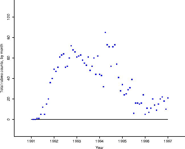
Figure 1: Rabies totals for the period of
the study, by month. Notice that by the middle of 1995 the number of rabid
animals per month has settled down to what appears to be a noisy but constant
level.
Wilson, et al. cite [9] in asserting that rabies in Connecticut has passed through the epizootic phase and entered an enzootic phase: ``... rabies in raccoons appears to have become enzootic in Connecticut, as has been observed elsewhere in the eastern United States following epidemic transmission.'' Has rabies indeed become endemic? Figure 1 shows the total numbers of rabid animals reported for the period from early 1991 to the end of 1996. In particular note that by the middle of 1995 the number of rabid animals per month has settled down to an apparently noisy but constant level, consistent with an endemic phase. These data were not available to Wilson, et al., but they saw the decreasing counts at the end of 1994 as indicating that the epizootic phase had ended, and the enzootic phase begun.
In addition, Figure 2 shows the results of a spatial statistical analysis on the clustering of onset of rabies cases. In particular, consider the data set consisting of the town areas on the map of Connecticut, and a binary (black and white) variable which is 1 if there was a case in the town in a given month, and 0 otherwise. Moran's I is a spatial statistic designed as a measure of spatial autocorrelation[7, 2]. As Moran's I becomes increasingly positive, neighboring areas are more similar to each other (the map shows increased clustering); as Moran's I becomes more negative, the map shows more dispersion (``hyperdispersion'': in the limit, the map looks like a checkerboard); when zero, the map will show both a lack of clustering and a lack of hyperdispersion.
Calculation of Moran's I for each month, using a spatial adjacency
matrix determined by spatial contiguity (the element ![]() corresponding to
towns i or j is 1 if two areas touch, and 0 otherwise)
corraborates the evidence contained in the total animal counts, that raccoon
rabies has indeed become enzootic in Connecticut. The statistic is essentially
zero at about the same point (mid 1995) at which the totals settle
down. Furthermore it sheds light on the perceived endemic phase from Figure
1: it could have been the case that, while totals are low,
they occur in clusters over the face of Connecticut. As it is, Figure
2 demonstrates that cases appear ``randomly'' over the face
of Connecticut.
corresponding to
towns i or j is 1 if two areas touch, and 0 otherwise)
corraborates the evidence contained in the total animal counts, that raccoon
rabies has indeed become enzootic in Connecticut. The statistic is essentially
zero at about the same point (mid 1995) at which the totals settle
down. Furthermore it sheds light on the perceived endemic phase from Figure
1: it could have been the case that, while totals are low,
they occur in clusters over the face of Connecticut. As it is, Figure
2 demonstrates that cases appear ``randomly'' over the face
of Connecticut.
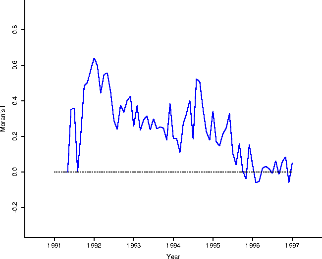
Figure 2: Moran's I calculated using the
spatial adjacency contiguity matrix (1 if two areas touch; 0 otherwise).
The characterization of the spread of rabies is addressed using the original data of Wilson, et al., plus data for the years 1995 and 1996. The most striking feature of their Figure 3 - from which they deduce the rate of spread - is the appearance of a wave moving from east to west. The first goal here is to model this wave. Figure 3 essentially replicates their figure (with the addition of two more years), showing time slices of the disease distribution using point plots for each quarter from 1991-1996. Wilson, et al. stated that ``...the epizootic front, albeit roughly defined, progressed at an average velocity of about 30 km. per yr., with occasional, isolated positive animals found beyond the front.'' The wave appears to have traversed all of Connecticut in only four years (the east-west distance of Connecticut is about 160 km).
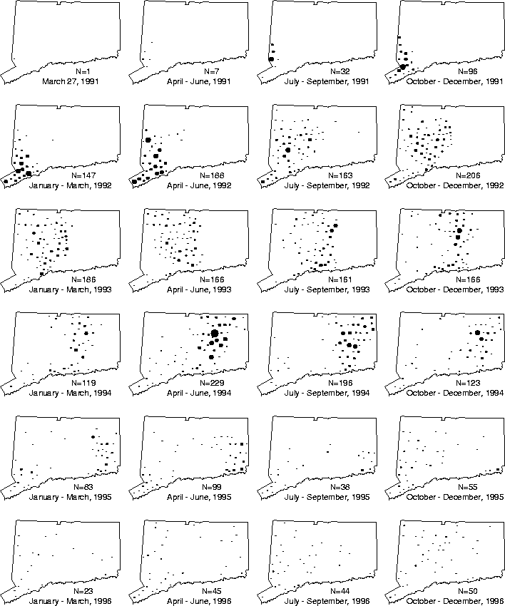
Figure 3: Time slices in the spread of rabies in
Connecticut (size of dot reflects number of animals).
To obtain estimates of the speed and direction of the epizootic front, consider the following model of time of first report of rabies as a linear function of space:
This model was fit to data comprised of centroids of each town and time (month measured from March, 1991) at which the first case was detected. Linear regression results in the equation
with an ![]() of 0.841 (where time is measured in months from March, 1991,
and space coordinates are measured in feet, using Connecticut State Plane
Coordinates of 1927). This model leads to an estimate of rate of spread of
46.0 km/yr, and provides an equation for the time of first report as a function
of centroid coordinates. We will treat it, however, as an equation for the
arrival of the epidemic front. The bias in this equation is obvious: it will
tend to be behind the actual arrival, as the disease could presumably go months
without detection prior to discovery of the first case.
of 0.841 (where time is measured in months from March, 1991,
and space coordinates are measured in feet, using Connecticut State Plane
Coordinates of 1927). This model leads to an estimate of rate of spread of
46.0 km/yr, and provides an equation for the time of first report as a function
of centroid coordinates. We will treat it, however, as an equation for the
arrival of the epidemic front. The bias in this equation is obvious: it will
tend to be behind the actual arrival, as the disease could presumably go months
without detection prior to discovery of the first case.
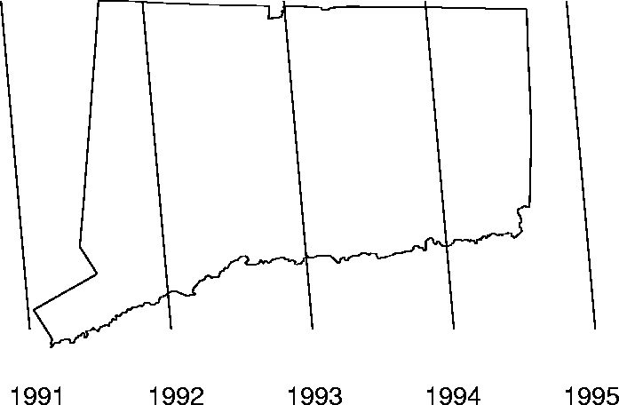
Figure 4: The front is modelled as a plane in
space and time. Cross sections of this line in space move from left to
right. The five lines for years 1991-1995 are represented here.
This model yields an estimate of a rate of spread of 46.0 km/yr, as opposed to Wilson, et al.'s estimate of 30 km/yr.
The coefficient of y is not significant at the .05 level (p=0.12): if y is dropped from the regression, regression leads to the equation
with an ![]() of 0.839, giving an estimate of a rate of spread of 45.4
km/yr. This represents a spread from east to west, rather than southwest to
northeast. We accept the first model, however, regardless of the
``significance'' of the coefficient of y, and use it in subsequent
analyses. Our objective is to establish the best fitting linear model, which is
given by the first regression. The front is shown in Figure
7. Note in particular the consequence of the bias mentioned
earlier: it appears that the epidemic actually kicks off many months before
actually modelled by the regression equation (Eq. 2).
of 0.839, giving an estimate of a rate of spread of 45.4
km/yr. This represents a spread from east to west, rather than southwest to
northeast. We accept the first model, however, regardless of the
``significance'' of the coefficient of y, and use it in subsequent
analyses. Our objective is to establish the best fitting linear model, which is
given by the first regression. The front is shown in Figure
7. Note in particular the consequence of the bias mentioned
earlier: it appears that the epidemic actually kicks off many months before
actually modelled by the regression equation (Eq. 2).
Wilson, et al. suggest that ``...little can be deduced concerning...whether the epizootic occurred uniformly throughout the region.'' They speak of ``local epizootic activity'': is it possible to characterize this activity? By synchronizing the towns to the epizootic front, we may be able to determine a ``typical'' response to the epidemic. This idea was inspired by Cliff and Ord[2], and, in particular, Figure 5.6(C) of their beautiful book.
Based on the front equation (Eq. 2), the objective is to model the effect of the epidemic at individual towns (the ``local epidemic''): there should be no cases prior to the arrival of the epidemic; cases would rise as the epidemic came to town; and one expects to see cases fall off to endemic levels following the passage of the epizootic wave.
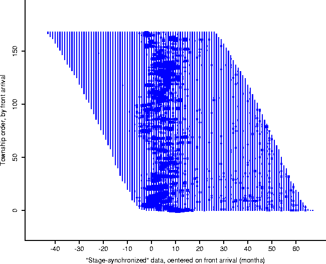
Figure: To calculate the form of the
local epidemic curve, the towns were stage synchronized to the same clock:
the arrival of the front, as computed by the front equation, Eq. 2.
In order to investigate this local activity, the towns were synchronized to the same stage of the epizootic, using the front as the master clock (Figure 5): that is, the town time-series were synchronized so that the cell corresponding to ``ground zero'' for each is at the same point (which we label 0); in this manner the time-series may be compared at corresponding stages in their local epidemics (Figure 6). Plotting the averaged animal values results in the form given in Figure 7.
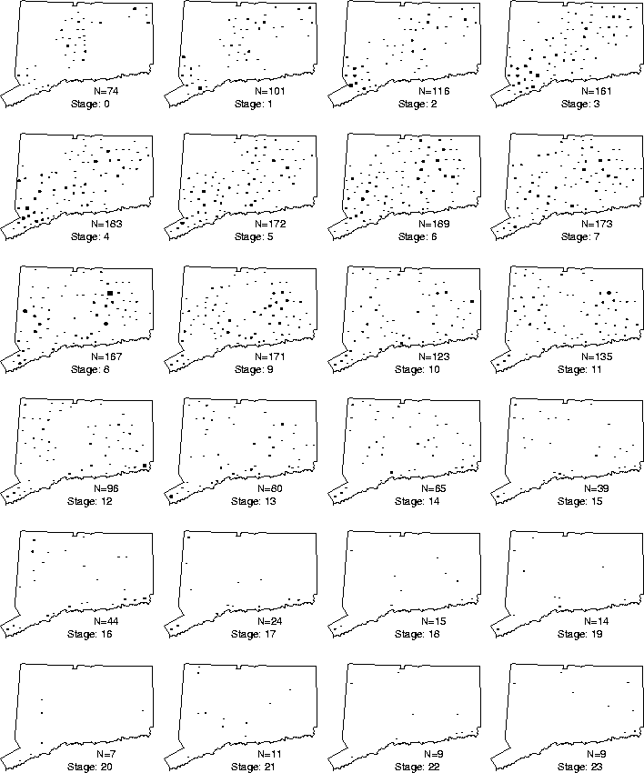
Figure 6: Stage slices in the spread of rabies in
Connecticut (size of dot reflects number of animals).
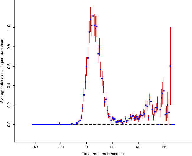
Figure: Averaged animal counts, plus or
minus one standard error, for towns referenced to common points in the
``local epidemic'' (the onset of which is modelled by the front in Figure
4). Towns on the western edge of Connecticut will appear
mostly on the right of zero (post-front): those on the eastern edge will show
relatively more of their series located to the left of zero (pre-front).
It appears that the epidemic actually begins a few months before expected by
the regression equation (Eq. 1).
Cliff and Ord[2] include a short study of the spread of fox rabies in Europe. They report rates of spread of from 30-60km/yr[3], consistent with this data. Furthermore, they discuss the form of the wavefront expected given the characteristics of rabies (especially the recovery rate of 0), which those authors call a ``Kendall wave'' of Type I (after Kendall[4]). The main spike of Figure 7 is remarkably consistent with this wave.
Notice that there is a precipitous drop after the initial spike of the epidemic to a strong depression, then what appears to be a consistent rise in rabid animals, ending in a degeneration into noisy reduced levels. One interpretation of this is as follows: as time goes on and the epizootic wave fades into the past, Wilson, et al. suggest that ``Following local epizootic activity, cases of positive raccoons declined rapidly. Because infection almost always leads to death[9], raccoon abundance probably was diminished, resulting in less infectious contacts and fewer new cases.'' As the population rebounds, rabies again takes a foothold, but keeps the population in check at a lower level with a steady rate of excess mortality above pre-rabies levels, all else being equal. The post-epidemic raccoon local populations rebound, but rise and fall subject to continued rabies re-infection (compare [3], Figure 1).
The synchronization among towns will be lost between regions and the front as time goes on, leading to an averaging of plots which are out of phase, resulting in a noisy appearance. Additional factors also muddy the waters: for example, Wilson, et al. describe this interesting mode of rabies spread: ``Unexpectedly, however, a focus of raccoon rabies appeared in northcentral Massachusetts during 1992, more than 100 km northeast of the Connecticut front at that time (Dr. Robert Deblinger, pers. comm.). An investigation there demonstrated that cases began at a landfill that served western Connecticut towns where rabid raccoons then were being reported. Garbage truck drivers reported that live raccoons regularly were found inside the refuse that they were dumping at this site.''
We modelled this waveform of Figure 7 with the function
(Figure 8), obtaining coefficients given in Table 1.
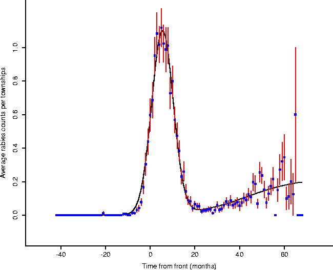
Figure: By fitting the model given by
Eq. 4, we obtain meaningful parameters (Table 1) which
characterize features of the local epizootic activity.
This function was chosen to represent the two phases of the disease: the epizootic (the first gaussian component), as well as the enzootic (the second sigmoidal component). While this model does not have any known basis in the underlying dynamics of the spread of rabies, it provides a convenient form for summarizing the characteristics of the form. For the epizootic component,
We briefly outline the status of our work on determining the form of the raccoon distribution. It is strictly preliminary, and may be substantially modified. One goal at this point is to create a better understanding of the assumptions necessary in order to derive an estimate of the population structure; the second will be the actual application to obtain the estimate, and that is still in the future.
There are, unfortunately, no data which would effectively provide a census of raccoons. The data used in this study were collected using a sampling procedure for finding rabid animals that was anything but optimal for the purposes of modelling one: as Wilson, et al. report, ``The recognition of animal cases in our study depended upon the presence, concern, and action of citizens and safety officials; therefore, results may not characterize the true extent or distribution of transmission.'' The data provide a biased sample, critically mediated by human population: where people are, there suspicious raccoons are discovered, killed, shipped to labs, and perchance declared rabid. In the absence of any human population, the number of rabid animals found would be zero; where population is very dense, every raccoon is shipped off to the state labs as a threat, and every rabid raccoon is be found. Reality is, as usual, somewhere between.
Wilson, et al. suggest that animals were not sampled evenly thoughout all regions, ``complicating analysis of the impact of the epizootic on animal demography.... Indeed, reliable data on raccoon density were not available, making it impossible to estimate the incidence of infection in the raccoon population or the demographic changes that may have resulted.'' Nonetheless, we are making the attempt. The price of modelling in the face of poor data is heavy assumptions, and we detail them below.
Assume that the pre- and post-epizootic raccoon population density
functions ![]() of raccoons are proportional: e.g.
of raccoons are proportional: e.g.
![]()
Our goal is to estimate ![]() (up to a multiplicative constant) by using
the rabid animal data. The upshot of this assumption is that the epizootic
swept past the towns, creating local
depressions in population; but once the wave had swept through the population,
the population structure
(up to a multiplicative constant) by using
the rabid animal data. The upshot of this assumption is that the epizootic
swept past the towns, creating local
depressions in population; but once the wave had swept through the population,
the population structure ![]() returned to its pre-epizootic state (up to a
scale factor). Is the spread of rabies analogous, perhaps, to a (small!) steam
roller passing over the raccoon distribution, flattening it out as it goes?
Does the steam roller treat all land use classes the same? Does it flatten
proportionally (all populations of raccoons cut in half, for example), or
selectively (urban raccoon populations decimated, forest populations
unscathed)? We assume that the density of raccoons may vary, but the
relative densities do not (e.g., if raccoons are twice as likely in deciduous
forest than in coniferous forest before the epidemic, then that ratio still
holds in the endemic phase).
returned to its pre-epizootic state (up to a
scale factor). Is the spread of rabies analogous, perhaps, to a (small!) steam
roller passing over the raccoon distribution, flattening it out as it goes?
Does the steam roller treat all land use classes the same? Does it flatten
proportionally (all populations of raccoons cut in half, for example), or
selectively (urban raccoon populations decimated, forest populations
unscathed)? We assume that the density of raccoons may vary, but the
relative densities do not (e.g., if raccoons are twice as likely in deciduous
forest than in coniferous forest before the epidemic, then that ratio still
holds in the endemic phase).
The toll of the disease appears to have been modest compared to the racoon population. Evidence for this is presented in Table 2 and shown in Figure 9. Trapper data rebounds to pre-epizootic levels at the end of the epidemic phase; nuisance reports climb prior to the epizootic, peaking during the epizootic. While there was a depression in total trapped animals over the epidemic period, it seems rather mild (and does rebound in the endemic phase).
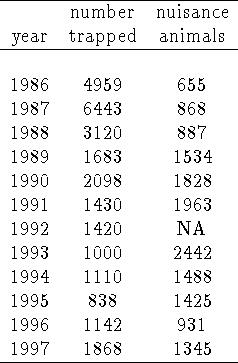
Table: Trapper and Nuisance animal data from Connecticut State
agencies. Refer to Figure 9 for a graphical depiction
of this data, in reference to rabid animal numbers.
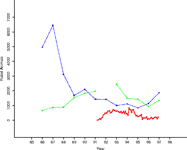
Figure 9: A clear impression of the
temporal progress of epizootic is given by this plot, summarizing our data:
trapper kills and nuisance calls (by year - the trapper numbers start higher),
and numbers of rabid animals (by month).
The salient point is that neither trapper data nor nuisance data is changed
dramatically during the period of the epizootic, preliminary
evidence that the population structure of the underlying raccoon population may
not have been radically altered during the period.
This data is suspect, of course, for the motivations of the trappers are unknown: were they encouraged to trap more animals during the epizootic, hence masking the actual precipitous drop in raccoon numbers? Were hunters avoiding the hunt due to their fears of rabid animals, resulting in a drop?
It is useful to introduce some additional data: land use information for the state[5], as shown in Figure 10 and broken down by category in Table 4. In addition to the data, we introduce some other assumptions:
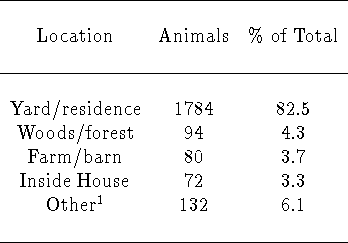
Table 3: From [8]: Location at which 2,162 rabies virus-positive
animals were found in Connecticut, 27 March, 1991 through 31 December,
1994 (a total of 361 cases were excluded due to inadequate information).
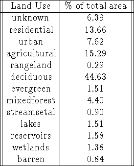
Table 4: Land Use categories used in this analysis
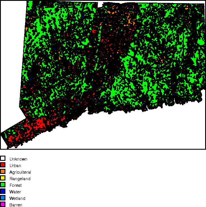
Figure 10: Land Use categories.
The model then takes the following form: let
Then we model ![]() as
as
That ![]() is a function of time and space is certainly troublesome;
but provided that in the endemic phase
is a function of time and space is certainly troublesome;
but provided that in the endemic phase ![]() , a constant,
then we can proceed (provided that we do all our rabies modelling in the
endemic phase), giving
, a constant,
then we can proceed (provided that we do all our rabies modelling in the
endemic phase), giving
where A is the matrix of land use areas ( ![]() ). Thus,
provided we can estimate
). Thus,
provided we can estimate ![]() , we can estimate
, we can estimate ![]() , as well as
the population of raccoons
, as well as
the population of raccoons ![]() : it is the sum of area types by size
times the density of raccoons by type of lulc,
: it is the sum of area types by size
times the density of raccoons by type of lulc,
The problem thus becomes to find ![]() .
.
If we limit ourselves to the data obtained during the endemic phase of
the study, which we consider to be late 1995, then the data is animal poor (15
months of few counts: Figure 11). In order to supplement
this set, consider the stage-synchronized data: this too would provide a
proportional surface for the rabid animal population, as once again in
Eq. 5 the rate ![]() is constant for the
stage-synchronized towns. Thus, while the constant may be different, the
stage-synchronized
is constant for the
stage-synchronized towns. Thus, while the constant may be different, the
stage-synchronized ![]() satisfies Eq. 6. The sum of the
two datasets thus also satisfies Eq. 6, with an adjusted
satisfies Eq. 6. The sum of the
two datasets thus also satisfies Eq. 6, with an adjusted
![]() .
.
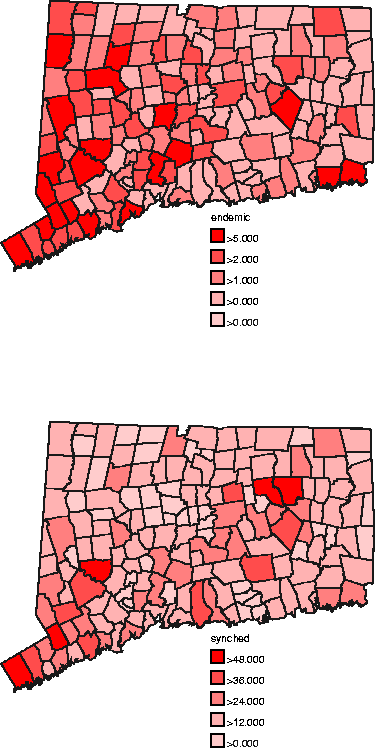
Figure 11: Top: endemic data; bottom:
epidemic stage-synchronized data. The endemic data was combined from time
slices for the period from late 1995 to the end of 1996. We included 15 months
worth of data from this period, yielding a total of 238 animals. The
correlation between population and this summed data is ![]() , a drop from
the reported
, a drop from
the reported ![]() of Wilson, et al. for the period through 12/94. The epidemic data
is summed from the 29 months of synchronized data for which all towns
reported.
of Wilson, et al. for the period through 12/94. The epidemic data
is summed from the 29 months of synchronized data for which all towns
reported.
Certainly one may wonder if these data sets may be combined: one is an average of time slices, the other an average of stage slices. One characteristic that we might test is the spatial autocorrelation of the stage-synchronized data: it should be small, just like the endemic data. Figure 12 assures us that this is so.
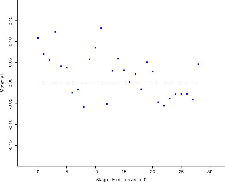
Figure 12: Moran's I calculated for towns
for the stage synchronized data (with numbers replaced by a binary variable
representing infected or not). The Moran's I values are small,
representing slight spatial autocorrelation (if any).
Human population density by land use type ( ![]() ) is obtained
using standard demographic variables and by projecting these onto the land use
map within the GIS GRASS. This information is crucial in the final analysis, as
one must account for the observers of rabid raccoons (without which no epidemic
would ever be declared!).
) is obtained
using standard demographic variables and by projecting these onto the land use
map within the GIS GRASS. This information is crucial in the final analysis, as
one must account for the observers of rabid raccoons (without which no epidemic
would ever be declared!).
Model the number of raccoons observed during this period for town i
of land use type T, ![]() , as
, as
![]()
where ![]() is an (undeterminable!) constant of proportionality. This says
that the number of rabid animals observed is linear in both raccoon population
and human population: if we double the number of raccoons the number of counts
doubles; similarly for the human observers. The solution vector
is an (undeterminable!) constant of proportionality. This says
that the number of rabid animals observed is linear in both raccoon population
and human population: if we double the number of raccoons the number of counts
doubles; similarly for the human observers. The solution vector ![]() is the density of rabid animals by land use, proportional to the true density
by land use.
is the density of rabid animals by land use, proportional to the true density
by land use.
Now solve for the d vector (up to a scale factor ![]() ),
),
![]()
where ![]() , to construct the total raccoon population
up to a constant of proportionality
, to construct the total raccoon population
up to a constant of proportionality ![]() , using Eq. 7.
, using Eq. 7.
The objective of this paper has been
The former objective has been met, yielding interesting and useful information: the rabies epidemic front proceeded at roughly 45 km/year, in a strong east-to-west fashion which was well modelled by a linear function of time as a function of space (Eqs. 2 and 3). Using this front, we were able to produce a clear signal of the local epidemic activity associated with the arrival of the epidemic front, the passage through the epidemic phase, and the transition to the endemic phase (Figure 4). This transition through the epidemic took on the order of 20 months. As to where rabies is moving now that the epizootic front is past, the disease is now endemic, and continues to appear ``haphazardly'' about the state (based on Moran's I calculations and the form of the local epidemic activity curve).
The latter objective shows a work-in-progress: we have tried to arrive at the fundamental assumptions and preliminary modelling techniques necessary to arrive at a reasonable model of the population distribution of raccoons from sparse data.
Acknowledgement: The authors gratefully acknowledge the contribution of Jay West, who prepared much of the data for this paper; Thomas Simon of the Animal Control Division, Connecticut Department of Agriculture, who helped in gathering and correcting data the original data; and Marie-Armande Calvo-Wilson, who assisted with the original data entry.
Financial support: Supported by a grant from the National Cancer Institute.