Model Prototypes

The model objects are organized into several prototypes, with the general prototype ="2D glim-proto=-1 inheriting from ="2D regression-model-proto=-1 , the prototype for normal linear regression models. The inheritance tree is shown in Figure 1 .

   
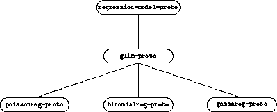
Figure 1: Hierarchy of generalized linear model prototypes.

This inheritance captures the reasoning by analogy to the linear case that is the basis for many ideas in the analysis of generalized linear models. The fitting strategy uses iteratively reweighted least squares by changing the weight vector in the model and repeatedly calling the linear regression ="2D :compute=-1 method.

Convergence of the iterations is determined by comparing the relative change in the coefficients and the change in the deviance to cutoff values. The iteration terminates if either change falls below the corresponding cutoffs. The cutoffs are set and retrieved by the ="2D :epsilon=-1 and ="2D :epsilon-dev=-1 methods. The default values are given by

> (send glim-proto :epsilon)
1e-06
> (send glim-proto :epsilon-dev)
0.001

> (send glim-proto :count-limit)
30

The analogy captured in the inheritance of the ="2D glim-proto=-1 prototype from the normal linear regression prototype is based primarily on the computational process, not the modeling process. As a result, several accessor methods inherited from the linear regression object refer to analogous components of the computational process, rather than analogous components of the model. Two examples are the messages ="2D :weights=-1 and ="2D :y=-1 . The weight vector in the object returned by ="2D :weights=-1 is the final set of weights obtained in the fit; prior weights can be set and retrieved with the ="2D :pweights=-1 message. The value returned by the ="2D :y=-1 message is the artificial dependent variable

constructed in the iteration; the actual dependent variable can be obtained and changed with the ="2D :yvar=-1 message.

The message ="2D :eta=-1 returns the current linear predictor values, including any offset. The ="2D :offset=-1 message sets and retrieves the offset value. For binomial models, the ="2D :trials=-1 message sets and retrieves the number of trials for each observation.

The scale factor is set and retrieved with the ="2D :scale=-1 message. Some models permit the estimation of a scale parameter. For these models, the fitting system uses the ="2D :fit-scale=-1 message to obtain a new scale value. The message ="2D :estimate-scale=-1 determines and sets whether the scale parameter is to be estimated or not.

Deviances of individual observations, the total deviance, and the mean deviance are returned by the messages ="2D :deviances=-1 , ="2D :deviance=-1 and ="2D :mean-deviance=-1 , respectively. The ="2D :deviance=-1 and ="2D :mean-deviance=-1 methods adjusts for omitted observations, and the denominator for the mean deviance is adjusted for the degrees of freedom available.

Most inherited methods for residuals, standard errors, etc., should make sense at least as approximations. For example, residuals returned by the inherited ="2D :residuals=-1 message correspond to the Pearson residuals for generalized linear models. Other forms of residuals are returned by the messages ="2D :chi-residuals=-1 , ="2D :deviance-residuals=-1 , ="2D :g2-residuals=-1 , ="2D :raw-residuals=-1 , ="2D :standardized-chi-residuals=-1 , and ="2D :standardized-deviance-residuals=-1 .