- Your exams are graded. You will have the opportunity to revise
them, to recover missing points.
Get me corrections/revisions by next Tuesday, and you'll get half the points back you correct. You're free to work together, and to discuss with me. Just fix things up, and we'll bisect perfect and your score.
If you don't mind, do the corrections on a new copy of the test (and you only have to do those that you didn't get right (or approximately right) the first time.
The mean and median now is 65. It will be at 82 if you all do your revisions....
Some comments:
- Hmmm.... I was a little disappointed by the Taylor series.
- Only 4 brave souls attempted this one! Recall that Hermite can be written as a Newton interpolating polynomial with those divided differences with repeated entries.
- Covered two pages, and a few of you didn't notice that the three
points in the difference table were supposed to be used
throughout. That was the major problem.
The second page of this problem used the parabola determined on the previous page, in Muller's method. And this was a simpler version of problem 5 -- looking for issues in secant method or Newton's method discovery of roots.
- I thought that this was the hardest one.
- Bisection doesn't care about the shape of the function -- concavity, differentiability -- it does require continuity.
- Think in terms of slopes, and regions. Then, most
importantly, what happens near 0?
Suppose that Newton is converging on
, and think about the ratio
.
I would have been satisfied with a graphic for this one, but a calculation is even better. As Lauren said, the derivative is "kinda yucky", and I agree....
Some used symmetry -- good!
Some of you focused on oscillations, but what else can go wrong?
- The secant one builds off of the Newton's method. Always ask yourself this: can I think of pairs that will give the desired solution? It's kind of like the bisection problem above.
- Sorry I haven't gotten your previous homework assignments graded
from last time. I had three tests to grade over the weekend,
and was sick in bed of grading poisoning. I'll have those for
you next time.
- I want to say a little bit about calculators, first.
- Also something about splines, from this
site:
Today we'll
- Look more at the errors in the simple rules,
- Talk about composite integration, and
- Think about adaptive quadrature.
- Section 7.2: simple quadrature rules
We want to evaluate
You encountered the following rules back in calculus class, as you may recall:
- Trapezoidal
- Midpoint
- Simpson's Rule
We actually usually start with left- and right-rectangle rules, and then consider the trapezoidal rule as the average of these. Simpson's can be considered an average of the trapezoidal and the midpoint rules.
As the authors point out, the first two methods (trapezoidal and midpoint) can be considered integrals of linear functions.
The trapezoidal method is the integral of a linear interpolator of two endpoints, and midpoint is the integral of the constant function passing through -- well, the midpoint of the interval!
This illustrates one important different application of these two methods:
- trapezoidal requires the endpoints;
- midpoint doesn't require the endpoints.
These methods are both examples of what are called "Newton-Cotes methods" -- trapezoidal is a "closed" method, and midpoint is "open".
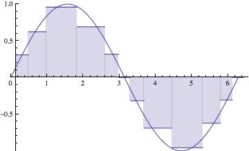
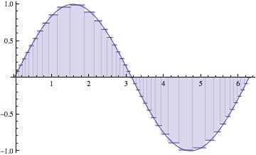
In the end we paste these methods together on a "partition" of the interval of integration -- that is, multiple sub-intervals, on each one of which we apply the simple rule. This pasted up version is called a "composite" rule.
We're going to start by assuming a partition of the intervalthat is equally spaced. But in the end, we should let the behavior of
help us to determine the the partition of the interval:


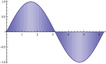
The maximum subinterval width ( ) goes to zero. The partition gets thinner and thinner, as the number of subintervals (n) goes to
.
The approximations get better and better, of course, as n) goes to.
Notice that the larger subintervals occur where the function isn't changing as rapidly.
This scheme would be called "adaptive", adapting itself to the function being integrated. That's what we're going to shoot for. - The derivation of the standard methods is carried out on pages
269-275, much as you might have seen before in calculus class.
Of particular interest in this section is the authors' very beautiful demonstration that Simpson's rule is the weighted average of the trapezoidal and midpoint methods.
In particular, that the midpoint method is twice as good as the trapezoidal method, and that the errors tend to be of opposite sign. This analysis is based off of an approximating parabola (see Figure 7.10, p. 271).
In that figure that bottom line is the tangent line at the midpoint (as suggested in paragraph above). The slope of that tangent line is actually equal to the slope of the secant line there, for a parabola. So the difference in those two slopes indicates the extent to which a parabolic model for
fails on that section.
First, let's compute the error for the Trapezoidal and Midpoint rules on a single subinterval (see p. 273). We should get the same result as we did by integrating the parabola.
Once we have those, we can determine what classes of functions each method will get exactly right: 7.3, 7.4, and 7.5 imply that
- Trapezoidal -- gets linear functions right
- Midpoint -- gets linear functions right
- Simpson's Rule -- gets cubic(!) functions right
Then we determine the error for the associated composite rules by just adding up the errors on the individual subintervals (p. 275).
Let's talk about how we might make this happen. I want to pursue a slightly different strategy from the one pursued by the authors. I'll give you a handout describing my strategy (but only after we've talke about it!).
By the way, the same ideas can be used to create plotting methods which are sensitive to the behavior of a function.