- Some of your homework assignments are graded:
- I was grading them this morning, and wondered why I had so few, then realized that some of you submitted them electronically.
- Unfortunately my NKU mail account only keeps a week's worth of emails, so I don't have them here on campus (but I do have them at home). So I'll finish the others tonight, and put them on my office door tomorrow.
- Some remarks:
- p. 179, #8: Some examples of O(h) -- Vicheth
- p. 190, #7 -- we talked about this the day before the exam. It was clear that folks didn't get the idea!
- p. 190, #4 -- I'll illustrate this (and the rest) with a Mathematica file
- You have a homework due next time, as well as your test revisions.
- I've also given you a short homework assignment, due Thursday
next. We may be able to start that today (it involves breaking the
adaptive quadrature code that we discuss today).
- For next time:
Please read the introductory section for ODEs (chapter 8). It's really quite a nice introduction (reminder) about why we're interested in solving ODEs, how to solve them analytically in a few cases, and a history of numerical solutions (dating back to the mid 1700s).
We'll be starting off with Euler's method next week, so you might read ahead into that section, too (in all of your spare time).
Today we'll
- Start with the errors in the simple rules,
- Talk about composite integration, and
- See how one might do adaptive quadrature.
- Section 7.2: simple quadrature rules
We want to evaluate
You encountered the following rules back in calculus class, as you may recall:
- Trapezoidal
- Midpoint
- Simpson's Rule
We actually usually start with left- and right-rectangle rules, and then consider the trapezoidal rule as the average of these. Simpson's can be considered an average of the trapezoidal and the midpoint rules.
As the authors point out, the first two methods (trapezoidal and midpoint) can be considered integrals of linear functions.
The trapezoidal method is the integral of a linear interpolator of two endpoints, and midpoint is the integral of the constant function passing through -- well, the midpoint of the interval!
This illustrates one important different application of these two methods:
- trapezoidal requires the endpoints;
- midpoint doesn't require the endpoints.
These methods are both examples of what are called "Newton-Cotes methods" -- trapezoidal is a "closed" method, and midpoint is "open".
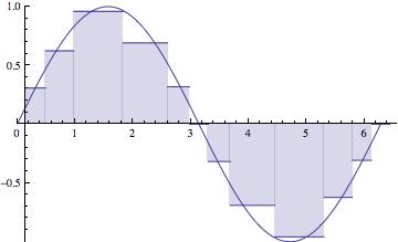
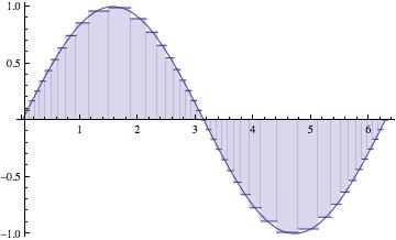
In the end we paste these methods together on a "partition" of the interval of integration -- that is, multiple sub-intervals, on each one of which we apply the simple rule. This pasted up version is called a "composite" rule.
We're going to start by assuming a partition of the intervalthat is equally spaced. But in the end, we should let the behavior of
help us to determine the the partition of the interval:


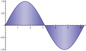
The maximum subinterval width ( ) goes to zero. The partition gets thinner and thinner, as the number of subintervals (n) goes to
.
The approximations get better and better, of course, as n) goes to.
Notice that the larger subintervals occur where the function isn't changing as rapidly.
This scheme would be called "adaptive", adapting itself to the function being integrated. That's what we're going to shoot for. - The derivation of the standard methods is carried out on pages
269-275, much as you might have seen before in calculus class.
Of particular interest in this section is the authors' very beautiful demonstration that Simpson's rule is the weighted average of the trapezoidal and midpoint methods.
In particular, that the midpoint method is twice as good as the trapezoidal method, and that the errors tend to be of opposite sign. This analysis is based off of an approximating parabola (see Figure 7.10, p. 271).
In that figure that bottom line is the tangent line at the midpoint (as suggested in paragraph above). The slope of that tangent line is actually equal to the slope of the secant line there, for a parabola. So the difference in those two slopes indicates the extent to which a parabolic model for
fails on that section.
First, let's compute the error for the Trapezoidal and Midpoint rules on a single subinterval (see p. 273). We should get the same result as we did by integrating the parabola.
Once we have those, we can determine what classes of functions each method will get exactly right: 7.3, 7.4, and 7.5 imply that
- Trapezoidal -- gets linear functions right
- Midpoint -- gets linear functions right
- Simpson's Rule -- gets cubic(!) functions right
Then we determine the error for the associated composite rules by just adding up the errors on the individual subintervals (p. 275).
Let's talk about how we might make this happen. I want to pursue a slightly different strategy from the one pursued by the authors. I'll give you a handout describing my strategy (but only after we've talked about it!).
The pictures we want to have in mind are on p. 298 (Figure 7.17) and p. 300 (Figure 7.19).
We'll use error analysis to help us decide if we're "close enough" to
the true value (within ).
The adaptive quadrature I consider would be called "local" rather than
global, because we don't sort the subinterval errors by size, and
attack the largest on the interval [a,b]. Instead we let each
subinterval work on its own turf, with its own chunk of the total error
.
By the way, the same ideas can be used to create plotting methods which are sensitive to the behavior of a function; we'll see that in my example code.