- This Friday: more Greatest Hits of the
KYMAA
- Today's climate news:
- The good:
- The bad:
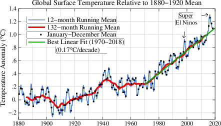
James Hansen and company publish a monthly update of global temperatures:

One thing I want to point out is their emphasis on the impact of El Nino. This is globally, of course, and it may not impact Togo as dramatically as the world at large.
Another thing is the apparently linear fit near the end. Maybe one could hope that it's linear there -- what do you think? But, even if so, it's moving at 1.7 degree per century...
- The good:
- Today's stereopticon of the day: more fun!
- The final project, updates:
- Thank you for your city reviews. I've returned my comments.
- These have been passed along to the modeling team, for their consideration.
- You noted some periods in your reports:
- Atakpame: 12, 16, 22
- Kara: 8, 12, 13
- Kouma: 28
- Niamtougou: 6, 8, 8.8?
- Lome: 1/5 year ($10 \pi t$)
- Tabligbo: 16
- Mango: 1/4, 8, 20, 24
- Sokode: 3, 7, 1.3, 1/4, 3.7
- Sotouboua: 16, 18
- There's still some confusion about periods: in \[ \sin(\frac{2 \pi t}{T}) \] the period is $T$ -- number of years in the cycle. The frequency is $\frac{1}{T}$ -- number of cycles per year. I'm a period person... but they're obviously pretty closely related!:)
- A reminder that if you have any Togolese data files out
on public websites, please remove them, or lock them down.
If you notice that I still have anything out and available, please let me know. You should access any Togo data you need off of the course website under the control of our data quality team.
- Matthew asked last time about other periods. I went a little crazy
with my homework, and, in particular, finally downloaded some
Sea Surface Temperature (SST) data (I averaged longitudes -4 to
6, and latitudes 0 to 6, using a website run by the Dutch: Climate Explorer).
Last time I told you that I'd tried incorporating ENSO (El Nino/Southern Oscillation), without much bang.
Some interesting results happened when I used SST.
- It drove the period 12 year oscillation out of the min temp and rainfall models (in that it was no longer significant at the .05 level).
- It drove the period 12 year oscillation out of the min temp and
rainfall models (in that it was no longer significant at the
.05 level).
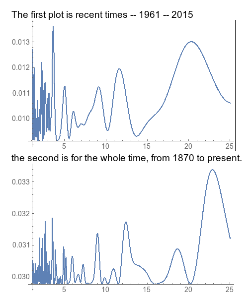
Some period views:

- It drove the linear year term out of the rainfall model(s) (in that it was no longer significant at the .05 level).
- It seems that SST itself is increasing with time as well
(regression analysis with the same sinusoidal components), so it may be
replacing the temporal component: SST
increasing. With SST in the model, increasing over time with a
positive coefficient, it will have the effect of increasing rainfall
with time.
- There is a reversal in the order of temporal impact on max and
min: min now increases 2.68 degrees per century, whereas max increases
only 1.37 degrees per century (directly). Again, both have a positive
dependence on SST, so if SST increases in time, so will the max and min
temperatures.
- There is a strong literature implicating SST in West African
rainfall: e.g.
- The Influence of Sea Surface Temperatures on African Climate
- West African rainfall deficits and sea surface temperatures
- Sea Surface Temperature Fields Associated with West African Rainfall Anomoly Types
And here are some papers related to temperatures and models in general:
- Asymmetric Trends of Daily Maximum and Minimum Temperature: "...the rise of the minimum temperature has occurred at a rate three times that of the maximum temperature during the period 1951-90..."
- Climate change uncertainty for daily minimum and maximum temperatures: A model inter-comparison
- Daily maximum and minimum temperature trends in a climate model
- Variability and Predictability of West African Droughts: A Review on the Role of Sea Surface Temperature Anomalies
- Thank you for your city reviews. I've returned my comments.
We're going to be working, as usual, with matrices, which represent transition between three classes:
- larvae (L),
- pupae (P), and
- adults (A).
- This Mathematica file gives us our introduction to the problem.
- A Leslie matrix is a matrix similar to a Markov matrix: a Markov
matrix can be a Leslie Matrix (but it need not be); similarly a Leslie
matrix may be a Markov matrix, but need not be.
\[
\left [
\begin{array}{ccccc}
{f_{11}}&{f_{12}}&{\ldots}&{f_{1,m-1}}&{f_{1,m-1}}\cr
{t_{21}}&{0}&{\ldots}&{0}&{0}\cr
{0}&{t_{32}}&{\ldots}&{0}&{0}\cr
{\vdots}&{\vdots}&{\ddots}&{\vdots}&{\vdots}\cr
{0}&{0}&{\ldots}&{t_{m,m-1}}&{0}
\end{array}
\right ]
\]
Unlike in a Markov chain, the transition components are not confined to
probabilities: the Leslie matrix is not a stochastic matrix, in general
(otherwise the sum of rows would be necessarily 1, and all transition
components would have to be 1!).
- A generalization of the Leslie matrix is an Usher matrix:
\[
\left [
\begin{array}{ccccc}
{f_{11}}&{f_{12}}&{\ldots}&{f_{1,m-1}}&{f_{1,m-1}}\cr
{t_{21}}&{t_{22}}&{\ldots}&{0}&{0}\cr
{0}&{t_{32}}&{\ldots}&{0}&{0}\cr
{\vdots}&{\vdots}&{\ddots}&{\vdots}&{\vdots}\cr
{0}&{0}&{\ldots}&{t_{m,m-1}}&{t_{mm}}
\end{array}
\right ]
\]
This is appropriate when individuals are in increasing size classes,
and may not return to a smaller class (but may "graduate" to the next
largest).
- In the end, it is a type of generalization of an Usher matrix that
we will use to study the flour beetle.
- I first implemented the essentials in this Mathematica file
- Of interest here is reproducing the dynamics, first of all. I frequently will read a book or paper next to the computer, where I attempt to recontruct figures and results.
- These results are particularly interesting to me for two
reasons:
- the dynamics (for such a simple system) are chaotic; and
- these extraordinarily complicated dynamics have been experimentally verified in the lab. This is the really impressive part.
- There are several parameters in this model. Remember that John von
Neumann famously said that "With four parameters I can fit an
elephant, and with five I can make him wiggle his trunk."
What can we do with six parameters? Evidently make the elephant dance chaotically....
I had to look up that quote, to see who said it. I discovered that von Neumann also wrote, in 1955, that "The carbon dioxide released into the atmosphere by industry's burning of coal and oil -- more than half of it during the last generation -- may have changed the atmosphere's composition sufficiently to account for a general warming of the world by about one degree Fahrenheit."
"In fact, to evaluate the ultimate consequences of either a general cooling or a general heating would be a complex matter. Changes would affect the level of the seas, and hence the habitability of the continental coastal shelves; the evaporation of the seas, and hence general precipitation and glaciation levels; and so on. What would be harmful and what beneficial -- and to which regions of the earth -- is not immediately obvious."
(Ironically, the title of his article is Can We Survive Technology?)
But I digress...
-
Let's talk a bit about the nature of the equations, and how
they are derived using those six parameters
\[ \begin{array}{ccl} {L_{n+1}}&{=}&{bA_n e^{-c_{el}L_n-c_{ea}A_n}}\cr {P_{n+1}}&{=}&{(1-\mu_l)L_n}\cr {A_{n+1}}&{=}&{P_n e^{-c_{pa}A_n}+(1-\mu_a)A_n} \end{array} \]
- What is $b$?
- What is $\mu_a$?
- What is $\mu_l$?
- What are $c_{el}$, $c_{ea}$, and $c_{pa}$?
As I mentioned, the key to the chaotic nature of the dynamics turned out to be the assumption (or rather the incorporation) of the dynamics of cannibalism!
This turns into the following "transition matrix" (notice that the entries are no longer constant, but functions of the population values): \[ \left[ \begin{array}{ccl} {0} &{0} &{b e^{-c_{el}L_n-c_{ea}A_n}}\cr {1-\mu_l}&{0} &{0}\cr {0} &{e^{-c_{pa}A_n}}&{1-\mu_a} \end{array} \right] \] and, as you can check, we have that \[ \left[ \begin{array}{c} {L_{n+1}}\cr {P_{n+1}}\cr {A_{n+1}} \end{array} \right] = \left[ \begin{array}{ccl} {0} &{0} &{b e^{-c_{el}L_n-c_{ea}A_n}}\cr {1-\mu_l}&{0} &{0}\cr {0} &{e^{-c_{pa}A_n}}&{1-\mu_a} \end{array} \right] \left[ \begin{array}{c} {L_{n}}\cr {P_{n}}\cr {A_{n}} \end{array} \right] \] Even though this appears to be a linear system, we must realize that the transition matrix no longer has constant coefficients: so it must be updated at every step.
If the system tends to a stable equilibrium, then so does the transition matrix, however: so we (will, next time) attempt to solve for an equilibrium, as we did for the wolves and moose.
- This
insightmaker model allows us to perform the same analysis. Let's
check that the Mathematica code and the InsightMaker model give the
same results in our first case.
- Your task: to use InsightMaker to reproduce the chaotic results of page 60.... The parameter values are at the bottom of the Mathematica file.