- I graded your quizzes, but it hurt (and I'm sure that some of you felt the same).
- I have an "almost key" made up of your good work. Let's take a look at that.
- A couple of comments:
- As I mentioned Friday, I included a problem which had been worked in the text (Example 3.65), as well as one of the homework problems. I want to encourage you to read your text and to do the homeworks, and one way that I can do that is by including those problems on quizzes. I will continue to do that.
- Please follow along with what I do during the daily agendas. That material, that we focus on in class, is fair game.
- Also as I said last Friday, if you try a homework problem and struggle with it, then you're welcome to ask about it in class (always good to give me a heads up if you can, so I'm ready for it -- but not required!), visit me during office hours, or just email a question or request a zoom.
- Just FYI: there is a distinction here between the formal and
informal definition of infinite limits. We will focus on the informal,
rather than the formal.
- I thought that I'd use some of the quiz problems to highlight a
few of the important ideas in this section.
The quiz featured four particular functions (or families of functions):
- arctan (featured in Example 4.21)
- arccos
- rational functions of the form \(\frac{1}{x^n}\), with \(n \in \mathbb{N}\) (one featured in Example 4.21)
- rational functions of the form \(\frac{ax+b}{cx+d}\), with \(c \ne 0\) (these are hyperbolas; also called Mobius mappings). An example is featured in Example 4.25, and another is the lead-off to the section.
- The section starts off with a Mobius transformation, or mapping,
Every rational function looks like a polynomial at \(\pm \infty\). This one looks like a constant function. Notice that we could rewrite it as \[ \frac{2x+1}{1x+0} \] which is of the form of the quiz function \(\frac{ax+b}{cx+d}\); and that the horizontal asymptote is the ratio of the leading terms. This is always the case when the degrees of the polynomials are the same.
We can go in the opposite direction: with \(c \ne 0\), we can rewrite \[ f(x) = \frac{ax+b}{cx+d} = \frac{\frac{a}{c}(cx+d)-\frac{ad}{c}+b}{cx+d} = \left(\frac{a}{c}\right) + \left(\frac{b-\frac{ad}{c}}{cx+d}\right) \] (you can see why it's important that \(c \ne 0\) in this analysis!).
- The first term on the right is just a constant, and is the value of the horizontal asymptote (and the ratio of the leading terms).
- The second term dies out (approaches zero) as \(x\) gets big (as \(x \to \pm \infty\)).
Hence the constant is the only term standing asymptotically.
When we do "asymptotic analysis", we're often interested in what happens to a function's graph when \(x \to \pm \infty\).
In the case of these functions, they look like constant polynomials as \(x \to \pm \infty\). They also have a vertical asymptote, wherever the denominator is zero (which is just the one point \(x=-d/c\) in this case). For this example, the domain might be given as \(\mathbb{R}-\{-d/c\}\): in other words, all real numbers except for the problem point.
- It's important that you realize that this is a general rule for
rational functions, however: Every rational function approaches a
polynomial as \(x \to \pm \infty.\)
The general rule is that the order of the polynomial is given by the ratio of the degrees of the polynomials that make up the rational function: if \[ r(x)=\frac{p_m(x)}{p_n(x)} \]
where \(p_m(x)\) is a polynomial of degree \(m\), and where \(p_n(x)\) is a polynomial of degree \(n\), with \(m \ge n\), then \[ r(x) \sim q_{m-n}(x) \] as \(x \to \pm \infty\), where \(q\) is a polynomial of degree \(m-n\). We read that \(\sim\) ("tilde") as \(r(x)\) "goes like" \(q\) as \(x\) goes to \(\pm \infty\).
If \(m < n\), then the rational function will go to 0 as \(x \to \pm \infty\).
It's actually easy to see what polynomial is the "asymptote". Let's do a couple:
- Here's one from the exercises: (Exercise 297):
\[
y=\frac{x^3+4x^2+3x}{3x+9}
\]
(degree 3 divided by degree 1, so the result will be
quadratic). We compute the limiting polynomial by long
division: does anyone remember that?:)
This is kind of a quirky example! But it should give you the general idea....
- Let's revisit the Mobius transformation,
\[
\frac{ax+b}{cx+d}
\]
And once we've done the division, let's re-write it to emphasize that it's just a transformation of the function \(\frac{1}{x}\).
- Here's one from the exercises: (Exercise 297):
\[
y=\frac{x^3+4x^2+3x}{3x+9}
\]
(degree 3 divided by degree 1, so the result will be
quadratic). We compute the limiting polynomial by long
division: does anyone remember that?:)
- The class of functions \(\frac{1}{x^n}\) are variations of this,
with \(n \in \mathbb{N}\). They're odd function if \(n\) is
odd, and even functions if \(n\) is even -- and no even
function is invertible on its domain. (Only trivial and
uninteresting "even" functions defined at the single point
\(x=0!\))
Their domains are \((-\infty,0) \cup (0,\infty)\), but the even powers and their inverses must be restricted to one half or the other.
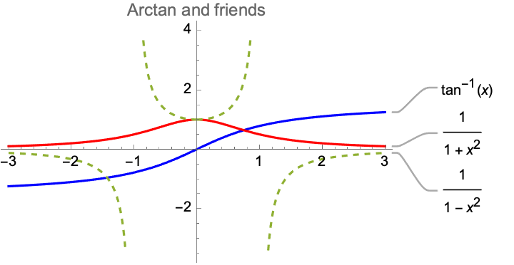
- Let's move on to the arctan function, also known as
\(\tan^{-1}(x)\) -- the inverse of the tangent function:
One comment is that in practice these functions always require an argument. That is we don't write "\(\tan^2\)" without the parentheses and a variable or value to be evaluated. For example, it's not permitted to write \[ \sin^2 + \cos^2 = 1 \] You have to provide an argument -- functions are hungry, and eat arguments: \[ \sin^2(x) + \cos^2(x) = 1 \]
Now for the quiz you were required to write the derivative of a composition of a polynomial (\(x^2\)) and the arctan function (which you do using the chain rule):
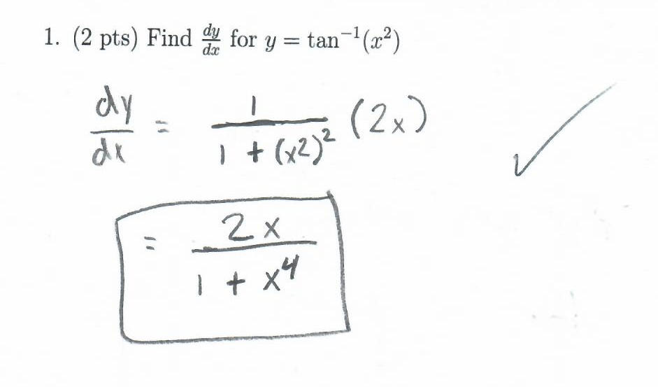
A few of you couldn't recall the derivative of the arctan function, and guessed that the derivative was \[ \frac{1}{1-x^2} \]
Looking at this graph of the arctan function, how do we know that this is incorrect?
An application of asymptotes shows that this isn't possible:
- the proposed derivative has vertical asymptotes (with dramatic consequences for the slope of tangent lines) -- but nothing very interesting is going on with respect to the tangent lines.
- Also the signs are wrong: arctan increases everywhere, so the derivative must be always positive.
- Furthermore the derivative must be small in magnitude, somewhere between 0 and 1.
- This guess gets the symmetry right, however: the arctan is an odd function, so its derivative must be even.
- Continuing on with the arctan function, let's consider what the
horizontal asymptotes tell us. In lab last Friday we were
considering a model for the growth of the population of New
York City.
We had population data through 1860, and fit an exponential function to it: \[ a b^t \] But we suspected that the model would break down in time, since it predicted a population of about 2 billion today...:)
In reality, we expect there to be a carrying capacity to the city's population. I pulled down some data to continue on from the previous data, and modelled it with two alternative functions: one is an arctan, \[ \frac{a \left(\tan ^{-1}(c (t-b))+\frac{\pi }{2}\right)}{\pi } \]
and the other based off an exponential (and called a logistic model):
\[ \frac{a}{1 + e^{c (b-t)}} \]
The three parameters do the same thing in each of these two models:
- \(a\): the carrying capacity
- \(b\): the location of the inflection point where it switches from concave up to concave down
- \(c\): scales the sharpness or speed of the switch from the lower horizontal intercept to the upper horizontal intercept.
- Mathematica on-line is an option, if you are at a computer without Mathematica installed. I've tried it and it worked pretty well!