Day 46 in Mat229

• The Brachistochrone Problem (1696, reputedly solved by Newton in a single day after he heard the challenge)
  

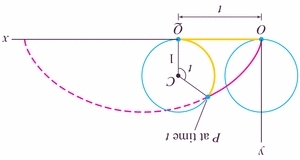
• The Tautochrone Problem (1673)

• inverting the equation \(x=f(t)\) to get \(t\) as \(t=f^{-1}(x)\), and then substituting \(t\) into the \(y(t)\) equation; or
• Finding a relationship between the formulas for \(x(t)\) and \(y(t)\) that eliminates \(t\).

In discussing parametric equations and curves, I made the point that parametric equations are useful for representing curves that cannot be represented as ordinary functions -- because the curves fail the vertical line test.

The most obvious example of this is a circle. It's so important, yet we can't represent it as a single function $y=f(x)$. We have to write, for example (and somewhat ashamedly) \[ y(x)=\pm\sqrt{r^2-x^2} \]

But if we think of it as a parametric equation, it's easy to write as a function of time -- as a motion -- just the way that you might trace it out on the board or on your paper: \[ \begin{array}{c} {x(t)=\cos(t)}\cr {y(t)=\sin(t)} \end{array} \] as $t$ varies over $[0,2\pi)$. That's if you like to start at (1,0), and draw in a counter-clockwise fashion. If you like to start at the top and go in a clockwise fashion (like time on a clock), then you might prefer \[ \begin{array}{c} {x(t)=\cos(\frac{\pi}{2}-t)}\cr {y(t)=\sin(\frac{\pi}{2}-t)} \end{array} \] as $t$ varies over $[0,2\pi)$....

In today's materials you'll see some pretty wild curves -- and even learn how to compute their lengths!

We'll also compute tangent lines to curves. In terms of motions, the tangent line is the path a particle would travel (initially) if whatever force is keeping the particle in its trajectory were to release. For example I often bring a weight on a string to class, and I'd be swinging a ball attached to a string over my head; and imagining along with you what would happen if one were to cut the string....

\[ \frac{dy}{dx} = \frac{dy}{dt}\frac{dt}{dx} = \frac{\frac{dy}{dt}}{\frac{dx}{dt}} \]

If you read along in our text, you'll see that, from the motion perspective, we are often more concerned with \(dx/dt\) and \(dy/dt\). However, it is often of interest to find out where a particle is at a particular point along the "backbone curve" \(y=f(x)\), along which the motion proceeds.

Let's think about uniform circular motion, for example, with \[ \begin{array}{c} {x(t)=\cos(t)}\cr {y(t)=\sin(t)} \end{array} \]

1. Where does the motion begin (i.e. where are we when \(t=0\))?
2. In what direction does the motion proceed?
3. If we cut the string how will the object fly away?
4. What is the slope of the tangent line anywhere (as a function of time)?
5. So how can we write the tangent line at a given moment in time?

Suppose we also want to compute the second derivative, \[ \frac{d^2y}{dx^2} \]

when faced with parametric equations $x=f(t)$ and $y=g(t)$.

It turns out to be just another application of the chain rule. The first derivative gets us started:

\[ \frac{dy}{dx} = \frac{\frac{dy}{dt}} {\frac{dx}{dt}} \equiv h(t) \] For the second derivative, we simply do it again -- but now we already know $\frac{dy}{dx}$ as a function of time (I called it $h(t)$ above), so \[ \frac{d^2y}{dx^2} = \frac{d}{dt} \left(\frac{dy}{dx}\right) \frac{dt}{dx} = \frac{\frac{d}{dt} \left(h(t)\right)} {\frac{dx}{dt}} = \frac{h'(t)} {\frac{dx}{dt}} \] It's a two-stage process. And obviously we could continue, computing third, fourth, etc. derivatives for the path in space.

• Calculus of Parametric Equations (.nb)
• Calculus of Parametric Equations (.pdf)