- Your homework is returned.
- Units! Don't forget them....
- That limit $\lim_{t\to\infty}\frac{\partial h}{\partial t}$ caused trouble....
- Tomorrow we'll continue working on new material, rather than Mathematica and exercises. We'll still have a quiz at the end of the hour.
- We'll have our first exam two weeks from today.
-
Just like univariate derivatives are closely linked to tangent lines,
which kiss a curve (osculate); about the slopes of those linear
approximations (tangent lines) to a univariate function; so are partial
derivatives are about slopes of univariate functions obtained by
slicing multivariate functions with planes. If the function is
differentiable at a point, then there is a tangent plane, which
kisses the surface.
An example from our author's TEC animations.
- Here's a Mathematica
file for similar problems which I stole from someone at the Air Force Academy....
- The tangent plane, provided it exists, is given by three points on
the surface (provided they're not co-linear). You can find three points
using the point at $(a,b)$, and points obtained by moving along the
cross-sections in the $x$ and $y$ directions.
The slopes in those directions are given by $f_x(a,b)$ and $f_y(a,b)$ as you set off from point the $(a,b)$.
If you take a one-unit step in either of those directions, the $z$-value would rise by either slope: \[ T(x,y)=f(a,b)+f_x(a,b)(x-a)+f_y(a,b)(y-b) \] If you take partial derivatives of $T$ at $(a,b)$, you will see that the partials (and the function value) agree with those of $f$ there.
- Strange things can happen, such as Example 4, p. 941. Let's take a look at
that one.
- #46, p. 944
- Use the limit definition to show existence
- Use two different approaches to show failure of continuity (limit doesn't exist)
- To finish this up, we turn to #45.
- #45: differentiability implies continuity; hence, if the function
of #46 is not continuous at (0,0), then it is not differentiable at (0,0).
- So, to wrap up #46, we show that the partials are not continuous at (0,0) (fail to have limits). If not, the function of #46 would be differentiable, and the linearization would be a tangent plane for the function. As it is, this function has no tangent plane at the origin.
To prevent problems, we introduce the following definition:
If $z=f(x,y)$, then $f$ is differentiable at $(a,b)$ if the increment $\Delta z$, which is the actual change in function values between the two points \[ \Delta z = f(a+\Delta x,b+\Delta y) - f(a,b) \] can be expressed in functional form as \[ \Delta z = f_x(a,b)(x-a) + f_y(a,b)(y-a) + \epsilon_1 \Delta x + \epsilon_2 \Delta y \] or \[ \Delta z = f_x(a,b)\Delta x + f_y(a,b)\Delta y + \epsilon_1 \Delta x + \epsilon_2 \Delta y \] where $\epsilon_1$ and $\epsilon_2 \to 0$ as $(\Delta x, \Delta y) \to (0,0)$.
We can generally avoid using this definition, however, because of Theorem 8, p. 942:
Existence and continuity of partials $f_x$ and $f_y$ are sufficient to imply differentiability.
That is, we can just check partials in two directions (but we require continuity of the partials for the function to be differentiable).
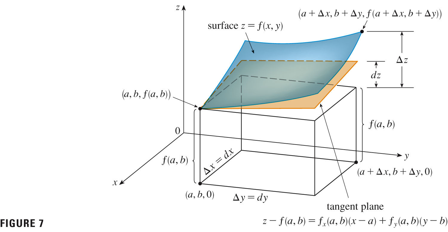
For a function $z=f(x,y)$, we define the differentials $dx$ and $dy$ to be independent variables; that is, they can be given any values. Then the differential $dz$, the total differential, is defined by \[ dz=f_x(x,y)dx + f_y(x,y)dy \] Differentials give us approximate changes to a function in the neighborhood of a point, generally when $dx$ and $dy$ are small, obtained by following along the tangent plane.
$\Delta{z}$ gives the actual change, so \[ \Delta{z}\approx dz=f_x(x,y)dx + f_y(x,y)dy \] The picture at the end of the section summarizes the situation nicely:
- #46, p. 944
- Let's take a look at the Discovery Project on p. 980, parts 1-3. This is
the natural extension of the tangent plane -- the tangent bowl.
- Why don't you carry out any analysis with a partner or two, and then we can check results with
- Some Mathematica code
- Here's a Mathematica
file for similar problems which I stole from someone at the Air Force Academy....
- We're generalizing the univariate chain rule: we start with a
function $y=f(x)$, where, in addition, $x(t)$. So $y$ is an implicit
function of $t$. If we want to know the rate of change of $y$ with
respect to $t$, we can do it in two steps:
\[
\frac{dy}{dt}=\frac{df}{dx}\frac{dx}{dt}
\]
or
\[
\frac{dy}{dt}=\frac{dy}{dx}\frac{dx}{dt}
\]
- In complete analogy, if we start with a
function $z=f(x,y)$, where, in addition, $y(t)$ and $x(t)$ are
univariate functions of $t$, then if we
want to know the rate of change of $z$ with
respect to $t$, we can do it in steps:
\[
\frac{dz}{dt}=\frac{\partial f}{\partial x}\frac{dx}{dt}+\frac{\partial f}{\partial y}\frac{dy}{dt}
\]
as mentioned in the text, we often write
\[
\frac{dz}{dt}=\frac{\partial z}{\partial x}\frac{dx}{dt}+\frac{\partial z}{\partial y}\frac{dy}{dt}
\]
instead.
The proof of this is actually easy to follow, and illustrates the use of the definition of differentiability. Let's take a look at it (p. 948).
For those of you in discrete math, why might we prefer a graph to a tree (e.g.
- There is a multivariate version of this: suppose that $x(s,t)$ and
$y(s,t)$. Then, when we look for a partial derivative of $z$
with respect to either $s$ or $t$ (since $z$ is a function of both):
\[ \frac{\partial z}{\partial t}=\frac{\partial z}{\partial x}\frac{\partial x}{\partial t}+\frac{\partial z}{\partial y}\frac{\partial y}{\partial t} \]
and symmetrically for $\frac{\partial z}{\partial s}$.
And of course we can do this for functions of any number of independent variables (the "General version", p. 951).
- We can gain some insight into implicit functions from our
univariate days using the ideas in this section. For example, an
implicit function, e.g.
\[
x^2+y^2=1
\]
which we recognize as the unit circle, can be reformulated as
\[
F(x,y)=x^2+y^2-1=0
\]
That is, we can think of it as a particular level curve (=0) of the
multivariate function \(F(x,y)=x^2+y^2-1\).
Applying the chain rule, we get \[ \frac{dy}{dx}=-\frac{F_x}{F_y} \]
Let's have a look at page 953, and think about the conditions under which we can do this (the Implicit Function Theorem). Why do they make sense, given our discussion of differentiability from last time?
Think about the linearization....
- Let's try a few simpler
exercises, and then move along to some of the more complicated
ones:
- #2, p. 954
- #7
- #15
- #37
- #38
- #49