Day 2, Mat128: Calculus A

The great thing about calculus is that it's really about straight lines! At least that much gets you a long, long way in calculus. So let's understand "line-like things" well....

\[ F = 1.8C+32 \] We've expressed this in "slope-intercept form", and it makes a certain amount of sense in this case (because the y-intercept -- \(C=0\) -- gives you the fahrenheit temperature of freezing): it's meaningful. But when it's not, this may be the worst form in which to express the relationship!

For example, suppose that we're looking at weight as a function of height, expressed in this case as \[ W=80+2H \]

Whoops! Someone got that equation wrong, didn't they?:) But let's suppose that they were right, and move along....

How much does one weigh when one is 0 inches tall?

80 pounds...:)

We do see the slope clearly from slope-intercept form, which tells us that for each additional inch in height, one predicts an additional 2 pounds in weight.

It's those first 0 inches that are killer! This illustrates that we are \(extrapolating\) in a part of the "domain" where the model breaks down completely -- the model is not useful there -- someone of 0 height is not of interest -- so why focus on the intercept? Notice that the y-intercept does not even appear on their graph, so why use slope-intercept form?

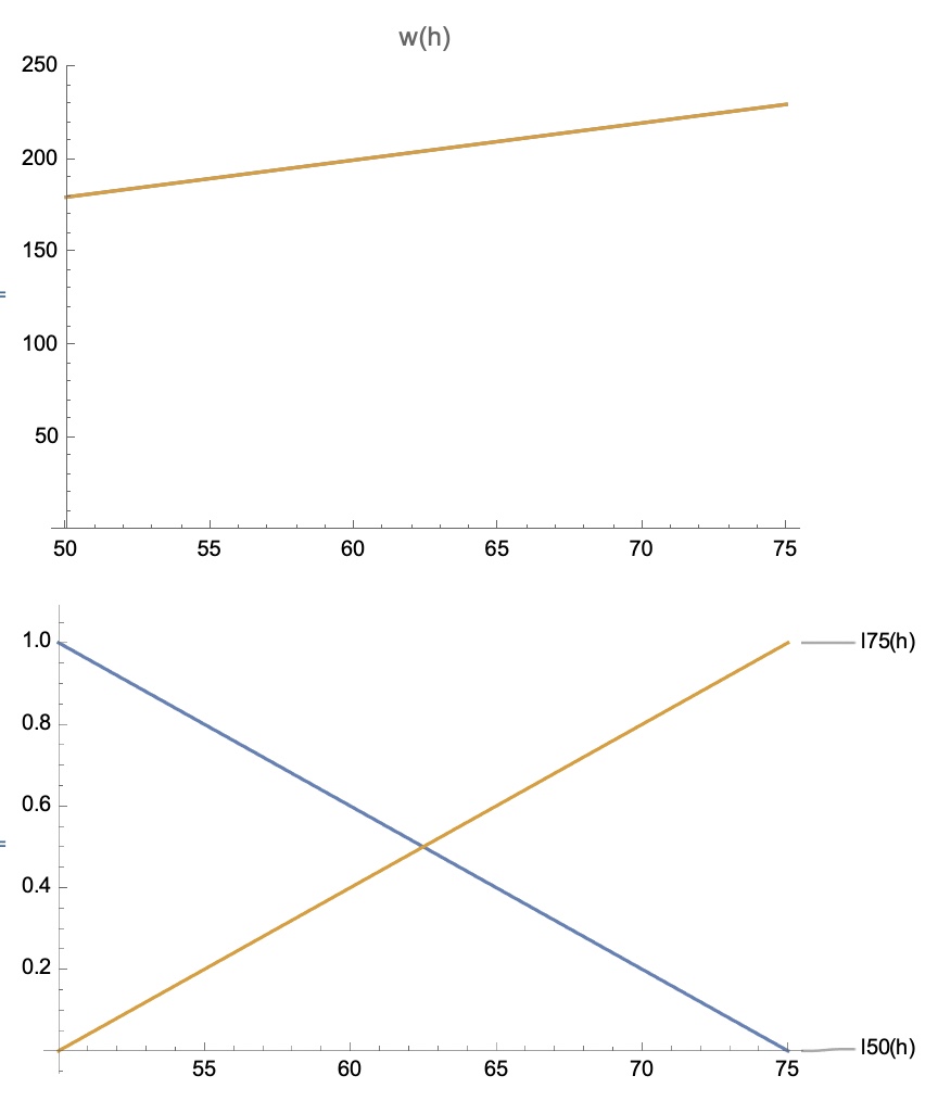
It would make a lot more sense to focus on the heights from about H=50 (W=180) to H=75 (W=230), say; and we can use those two points and this equation to re-express the relation using point-point form (reducing to point-slope form) as \[ W = \frac{230-180}{75-50}(H-50)+180 = 2(H-50)+180 \] From point-point form, we can see at a glance that \(W(75)=230\), and that \(W(50)=180\). From point-slope form, we can only see that \(W(50)=180\)....

This form of the equation is asymmetric: why focus on the height of 50, rather than 75? Why not write \[ W = \frac{180-230}{50-75}(H-75)+230 = 2(H-75)+230 \] At a glance we can see that \(W(75)=230\). But now 50 is murkier....

A method due to Lagrange is much more symmetric, and presents the line in such a way that one can see the weights at the two points easily: \[ W = 180\left(\frac{H-75}{50-75}\right) + 230\left(\frac{H-50}{75-50}\right) \] Note that the weight for height 50 is the coefficient of the \(H-75\) term, and vice versa.

Those two linear terms \(\frac{H-50}{75-50}\) and \(\frac{H-75}{50-75}\) are specially crafted so that they are 0 at one point, and 1 at the other:

You might think "Holy smokes, we've sure complexified that first equation!" (and you'd be right): but we do it for a reason. For one thing, the Lagrange method can be generalized to fit not just two points, but to fit an arbitrary number of points! (A quadratic function can fit three points, a cubic function can fit four, etc., and the Lagrange idea generalizes easily to do this.)

It also gives us another way to think about that line relating weight to height: as we slide from 50 to 75 in height, the predicted weight slides from 180 to 230.

It's easy enough to check that each of these functions give the same graph: if they give the correct weights at the two heights 50 and 75, then, since there is only one line that passes through the points \[ (50,180) \textrm{ and } (75,230) \] this must be a valid equation of the line....

In general, in calculus, the most useful form of the linear equation will be the point-slope form: given slope \(m\), and point \((x_0,y_0)\),

\[ y - y_0 = m(x-x_0) \] or \[ y = m(x-x_0) + y_0 \]

The value of \(m\) will frequently be given by what we will call the derivative at \(x_0\): \[ m = f'(x_0) \]

1. Linear versus affine....
2. Something about inverse functions....
3. More on linear versus affine
4. Three forms of linear equations
5. Finally -- slope! And linear models....