- Roll
- You have an assignment for next time: please prepare!
- A reminder that this (and the last Friday) are the only two without some assessment taking place. No quiz this week, but we'll start in on them next week.
- No class Monday, in celebration of MLK, Jr. Day.
- We talked about the various forms for functions with straight line graphs. You should be familiar with
- slope-intercept form
- point-slope form
- point-point form
- I also talked about the symmetric Lagrange form, e.g.
\[
W = 180\left(\frac{H-75}{50-75}\right) + 230\left(\frac{H-50}{75-50}\right)
\]
and, although I said that I wouldn't be saying much more about
it, let's say goodbye with just three more observations:
- It doesn't show you the slope, as the other three do (that's why it's not so good for calculus!);
- It's focused on the points fit by the line instead. I just
want to illustrate it in action, with more points: the use of
the Lagrange linear forms to fit multiple points.
Quadratic and Cubic (and higher) fits are created from Lagrange linear forms. Once again, the power of linear things....
- Lagrange
was a very important physicist: "Lagrange's treatise on
analytical mechanics,... written in Berlin and first published
in 1788, offered the most comprehensive treatment of classical
mechanics since Newton and formed a basis for the development
of mathematical physics in the nineteenth century."
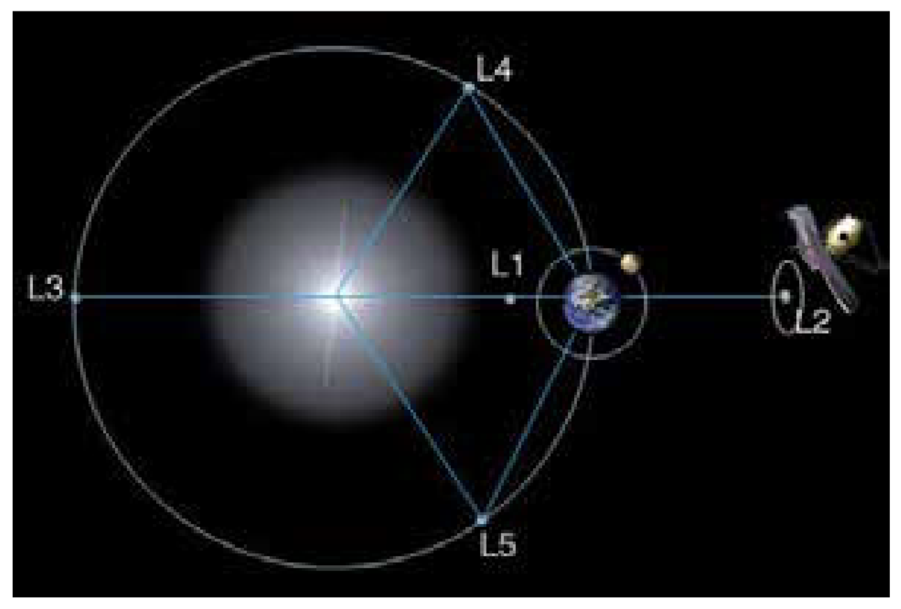
I was inspired to revisit this because of an article in the Fall, 2023 Radiations magazine, about "Lagrange Points". Turns out there are five points in a two-body astronomical system at which a satellite, placed in orbit there, would remain stationary, and not tumble into either body. The James Webb telescope is sitting at one of these points as we speak!

If you'll check out this article, you'll notice that calculus is the key to showing that there are five such points, as well as locating them.
In general, in calculus, the most useful form of the linear equation will be the point-slope form: given slope \(m\), and point \((x_0,y_0)\),
\[ y - y_0 = m(x-x_0) \] or \[ y = m(x-x_0) + y_0 \]
The value of \(m\) will frequently be given by what we will call the derivative of \(f(x)=y\) at \(x_0\): \[ m = f'(x_0) \] This we can think of as the instantaneous rate of change of the function \(f\) at that point. So let's talk about rates of change...
- You should have noticed all the straight lines!:)
- The key concept presented in section 1.1 is average
velocity:
\[
AV_{[a,b]} = \frac{s(b)-s(a)}{b-a}\text{.}
\]
which is the slope of a secant line,
\[
\frac{rise}{run}
\]
But the really interesting notion is instantaneous velocity! That's where calculus comes in.
The key to instantaneous velocity is something called an "indeterminate form", and limits. We'll get a look at that in the activity we do next, but it's hinted at by thinking about average velocity: it's defined by slopes, a change in \(y\) over a change in \(x\) (which we can think of as "rise over run"):
\[ AV = \frac{\textrm{change in y}}{\textrm{change in x}} = \frac{\Delta y}{\Delta x} \]
Now what happens as that "change in \(x\)" approaches 0? (that's the "limit" part: \(\Delta x \longrightarrow 0\))
If all is well in the world, then the ratio becomes indeterminate because the "change in \(y\)" also approaches 0! And everyone knows what \(\frac{0}{0}\) is, right?
(Just kidding -- that's the "indeterminate" part!) Watch as \(\Delta x \longrightarrow 0\) here:
In this case, however, "\(\frac{0}{0}\)" works out to the slope of that tangent line at the point \((a,f(a))\).
For the moment, however, we're going to follow our author's suggestion, that "The instantaneous velocity of a moving object at a fixed time is estimated (my emphasis) by considering average velocities on shorter and shorter time intervals that contain the instant of interest."
- Of course we should look over the Preview
activity.
I hope that you took the time to attempt that.
I'm going to have you partner up to compare your previews. Then we'll go over the "solution".
- Let's have a go at one of the activities from the section
(1.1.2),
during which we'll try to make sense of these notions.
We'll combine it with a trick from Example 1.1.2, however, to make the calculations easier: \[ AV_{[a,a+h]} = \frac{s(a+h)-s(a)}{h}\text{,} \] We're computing AV over and over again, so let's use the expression for \(s\) (and Algebra!:) to simplify things (algebra is actually supposed to help you make your life easier):
\[ AV = \frac{\textrm{change in y}}{\textrm{change in x}} = \frac{s(0.8+h)-s(0.8)}{(0.8+h)-0.8} = \frac{\hspace{3in}}{h} \] Now what?
- Then it's on to today's group activity, which involves solidifying
your understanding of these issues (including units). Your
worksheet for today.
If you don't finish this in class, then finishing it becomes part of your homework, and we'll review on Wednesday, next week.
- Notes from today: using algebra to remove indeterminacy in AV
