Math Modeling: Day 35

1. In-class portion:
   1. In-class exam
   2. In-class key
   Your in-class exams are graded -- but I have not yet put them into your directories. (Let me know if you're still having trouble accessing your directory.)

   Your exams are uploaded now. (I didn't want to do that while some of you were still doing your take-home -- I thought that it might be a distraction.)

   I'll hold off on a curve until I grade the take home. Mean (so far) is a 74, median 77.

2. take-home portion:
   1. Take-home exam

   2. Take-home exam non-linear model fit (Mathematica code)

      These were still coming in late last night -- haven't had a chance to look at them yet. I'l hope to have them graded by Wednesday.

But it is clear that we need to focus on solidifying some of the basics before moving on to more interesting topics (e.g. simulating the data, and trying to compute the probability of Fletcher's results, given a null hypothesis of no climate change). So, much as I hate to say it, I think that I must put that on the back burner.

So the question becomes, what goes on to the front burners?

And the answer is....

I went back to NOAA, and tried a few tricks -- and this time I came up with the Bowling Green data, which, coincidentally, started in 1893! (If you try that NOAA link, use zip code 43402).

So, with the two weeks we have remaining, I want to build a few linear (or non-linear) regression models for the Bowling Green data.

It won't be an exciting finish, but hopefully it will emphasize some points.

1. One of the things that struck me the most about the exam was your comments about Fletcher and climate change. At least half of you thought that Fletcher was on board with climate change, when, in fact, he a) never mentioned it, and b) explicitly denied that he thought that it was happening (without using those words). He thought that the climate of Wood County (as represented by temperatures in Bowling Green) would continue pretty much as it had for the previous 140 years or so.

2. Given that most of you hadn't picked up on this, my presumption was that you mostly weren't invested in the project. It was, I must say, front and center of the reading that I'd assigned from my work so far on the Fletcher project (first paragraph of the first page of the reading):

   While describing significant weather events since the founding of Wood County, he remarks "At that time, some weather followers believed in the occurrence of quadri-gesimal winters, or cold blustery winters in a forty-year cycle with cold winters every twenty years capped off by severe winters every forty years. The year 1780 had produced heavy snow and severe cold in Kentucky with severe flooding; this occurred again in 1800 and 1820, not only in the Great Lakes region but from the Mid-Atlantic states to New England. Severe weather again visited Wood County in 1841 and 1842, but the author believes in only irregular weather cycles." [My emphasis]

   Now I must say that it breaks my heart, to be honest, that I've had such little buy-in to the projects that we've studied this year. There are lots of reasons (at this moment in history) that you might be distracted; but, to be honest, I was noticing a certain lack of focus even before we went to spring break....

   But, as I am found of quoting from Doris Day, "Que sera sera."

   So: how to wrap up?

3. Another thing that occurs to me, as I look over these exams, is that many of you are willing to look at a model -- let's just call it a non-linear model -- without actually looking at it -- its form, or its diagnostics (which tell us if it's even a plausible model).

   I asked you to explain the form of a model chosen, and asked you to comment on (to evaluate -- remember UPCE?) the fit -- and some of you could not get started (even though I asked you to "fill the page..."). So that's a point of weakness. Two questions: 1. why choose the form we do, and 2. how do we assess whether the model is good or not? That's a destination, and we should be able to arrive there before the end of the term. That, at least, would be good.

   Let's talk about model form, and about fit. And let's talk specifically about the Procter and Gamble problem from the exam (fraction of Chlorine).

   1. Model form: some of you thought that a dying exponential was appropriate. Good! That's an excellent start; but it's not the end.

      The model was written in an unusual form. The easiest way to write a shifted dying exponenial would be \[ chlorine(t) = \alpha + \gamma e^{-\beta t} \]

      $\alpha$ represents the horizontal asymptote; $\gamma$ the total change in fraction over time; and $\beta$ determines the speed with which the product makes that change. Each term plays an important role; each term is interpretable.

      But they wrote the chosen dying exponential in an unusual fashion: \[ chlorine(t) = \alpha + (0.49 - \alpha) e^{-\beta (t-8)} \]

      The two models are not equivalent -- there is more freedom in the former, because we haven't constrained the function to take a particular value, as we have in the latter case. There are three free parameters in the first model, but only two in the second.

      In the latter case, the shift by 8 represents 8 weeks, and we can see that if we put $t=8$ into the equation, then $chlorine(8) = 0.49$.

      So this model is specifically constructed so as to interpolate a known value of chlorine -- the eight week value. We've imposed an important constraint upon the model. We've tied its little model hands....:)

   2. Now: having chosen the simpler exponential model, we might ask how good is the fit compared to the linear model?

      Some of you "took the bait" during the exam, and fell for Mathematica's non-linear $R^2$. But, as I told you in class, non-linear regression values of $R^2$ are not equivalent to the $R^2$ of linear regression model -- and some very reasonable statisticians don't think that we should consider them at all!

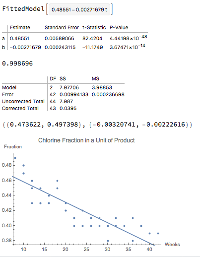
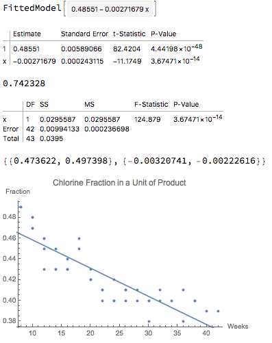
      To prove it to you, let me observe that we can obtain the linear model for chlorine using either linear regression or with non-linear regression(!):

      			lm = NonlinearModelFit[data, a + b * t, {a, b}, t] 
      			lm = LinearModelFit[data, t, t]
      			

      Using non-linear regression is killing a fly with a cannon, but we can do it. Both produce the same model, but not equivalent diagnostics: observe the difference in the $R^2$ values presented.
      

      The models are identical -- they're just obtained using different processes -- and yet one says that the $R^2$ is .74 or so, whereas the other says it's .999.... The $R^2$ values are not comparable.

      Notice that the confidence intervals are the same.

   3. One thing that many of you did not comment on was the confidence intervals. CIs are really important. As I tried to emphasize earlier in the course, the values we obtain for the parameters are wrong -- not because we're stupid or evil, but because there's error in data, etc. -- which causes our values to come out wrong. They're estimates. We do, however, have confidence intervals, which tell us that the true values are in an interval (with given confidence). So you have confidence (say 95%) that the true value of the parameter is in a box -- but also we should have confidence that 5% of the time we're wrong again -- and that it's not in the box!

      It's good to talk about that parameter value, that "best value", which the regression returns: we may want to use it to give a "ballpark figure" to whatever it happens to represent (e.g. the number of degrees of temperature per year that the DTR drops); but it's important to keep it within the context of the box.

      For example, when you were looking into the DTR problem prior to the exam, I asked you to find a model -- but the really important question was not the actual value of the slope obtained, but rather the fact that it was significantly different from 0 -- 0 is not an element of the CI -- and negative -- which says that the DTR is actually getting smaller (in accord with predictions and other data collected around the world).

      What would Lyle Fletcher say?! I wish that we could have that conversation. I'm hoping that he would say "That's really interesting, and wonderful (and scary). What else can statistics tell us about the climate of Wood County?"

      But he might just dig in and say "Fake news!"....

1. We can now check Fletcher's dates. Can you construct a new data set that has the years of temperature extremes? For each day of the year, we want to know which year had the max max, the min max, etc.

2. Can you construct a model of the form \[ \alpha + amp Sin[2\pi (t - phase)] \] for the maximum temperatures (where $t$ is in years), for the minimum temperatures, and for DTR?

   What if we add a linear term: \[ \alpha + \beta x + amp Sin[2\pi (t - phase)] \]

   And remember: it's not just the values of the parameters, but also the significance of the parameters -- is it possible that they are zero? In which case we can drop that portion of model from consideration....

   To evaluate the effectiveness of a model, it might pay to focus on the mean square residual: that seems a fairer metric for evaluating the difference between models (and one that I'd hoped you'd focus on during your exam -- I emphasized it by actually doing that calculation separately, even though it already figured in the tables of regression results).